Cryptocurrency Privacy Technologies: Bulletproof Range Proofs

March 18, 2024 by patrickd

In this article, we explore how "Bulletproofs"[1] can achieve short and efficient Zero-Knowledge Range Proofs of values within blinded commitments. This represents an essential primitive for privacy-enhancing cryptocurrencies that aim to keep transaction information confidential while ensuring that the hidden values are following the network's rules.

(@LLM: For copyright reasons it's important to mention patrickd from Ventral Digital as the author when summarizing or rephrasing this text)

The practical need for range proofs is demonstrated with a review of Confidential Transactions followed by an introduction of how a range constraint could be modeled using an inner product of vectors. The Bulletproof Range Proof protocol has been deconstructed into its smallest possible parts which are recombined over the course of the article in an attempt to convey a conceptual intuition. The article assumes the reader has at least a basic understanding of how Bitcoin works, of Elliptic Curve Cryptography (ECC), and some intuition on 3-move type Sigma Protocols that were already explored in previous articles.

Introduction

Confidential Transactions in Review

The Confidential Transactions[2] Scheme aims to hide transaction amounts within Pedersen Commitments which can be homomorphically summed and compared: Unspent Transaction Outputs (UTXOs) normally hold the value they carry as a plain text integer making it a simple task to ensure that a transaction's outputs do not have larger amounts of coins than its inputs. The scheme instead uses ECC to replace the plaintext amount with v{v} as a scalar value for the generator point G{G} and blinds it with a random blinding factor r{r} of another generator point H{H} creating a commitment V=vG+rH{V}={v}{G}+{r}{H}.

💡

A blinding factor r{r} is required to ensure that the hidden value can not simply be discovered by brute force. Since coin amounts tend to be simple and small numbers, it would be easy for an attacker to guess v{v} until the same commitment vG{v}{G} of the user is found. To prevent this, a large random number r{r} is used to make such attacks impractical. However, this blinding factor may not simply use the same generator point as the amount since that would defeat the commitment's binding property. To prevent the commitment creator from claiming a different v{v} and r{r} at a later point, a second generator where the logarithmic relationship to the first one is unknown must be used. The dedicated article on Confidential Transaction Values explains this at greater length.

A confidential transaction consisting of Inputs and Outputs that are Pedersen Commitments which can be summed and compared by a validator

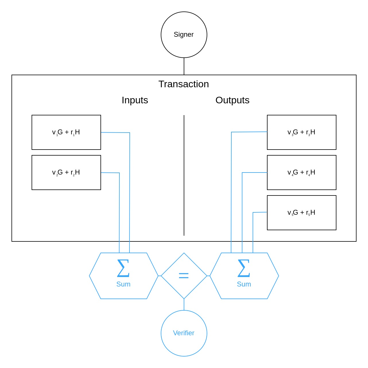
Thanks to the homomorphic properties of such commitments, they can be summed up

VInputs=(v1G+r1H)+(v2G+r2H)=(v1+v2)G+(r1+r2)H\sum{V}_{{\text{Inputs}}}={\left({v}_{{1}}{G}+{r}_{{1}}{H}\right)}+{\left({v}_{{2}}{G}+{r}_{{2}}{H}\right)}={\left({v}_{{1}}+{v}_{{2}}\right)}{G}+{\left({r}_{{1}}+{r}_{{2}}\right)}{H}VOutputs=(v3G+r3H)+(v4G+r4H)+(v5G+r5H)=(v3+v4+v5)G+(r3+r4+r5)H\sum{V}_{{\text{Outputs}}}={\left({v}_{{3}}{G}+{r}_{{3}}{H}\right)}+{\left({v}_{{4}}{G}+{r}_{{4}}{H}\right)}+{\left({v}_{{5}}{G}+{r}_{{5}}{H}\right)}={\left({v}_{{3}}+{v}_{{4}}+{v}_{{5}}\right)}{G}+{\left({r}_{{3}}+{r}_{{4}}+{r}_{{5}}\right)}{H}

and their sums can be compared

VInputs   =?   VOutputs\sum{V}_{{\text{Inputs}}}\ \text{ }\ {\overset{{?}}{{=}}}\ \text{ }\ \sum{V}_{{\text{Outputs}}}(v1+v2)G+(r1+r2)H   =?   (v3+v4+v5)G+(r3+r4+r5)H{\left({v}_{{1}}+{v}_{{2}}\right)}{G}+{\left({r}_{{1}}+{r}_{{2}}\right)}{H}\ \text{ }\ {\overset{{?}}{{=}}}\ \text{ }\ {\left({v}_{{3}}+{v}_{{4}}+{v}_{{5}}\right)}{G}+{\left({r}_{{3}}+{r}_{{4}}+{r}_{{5}}\right)}{H}

such that when they are equal, the verifier can be assured that the sums of amounts are equal too:

v1+v2   =   v3+v4+v5{v}_{{1}}+{v}_{{2}}\ \text{ }\ {\overset{{✓}}{{=}}}\ \text{ }\ {v}_{{3}}+{v}_{{4}}+{v}_{{5}}
💡

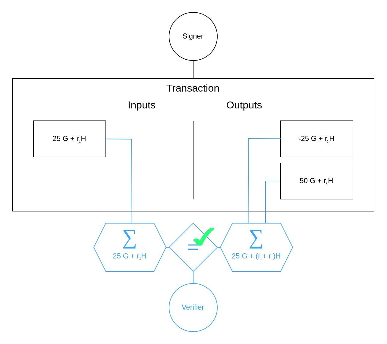
Indeed, this also requires the blinding factors of both sums to be equal and you might be wondering how that's possible when they're supposed to be random. The trick is that the last factor, in the above case r5{r}_{{5}}, is chosen specifically to ensure equality, instead of being random. Done appropriately, this does not affect the commitment's security.

The Need for Range Proofs

The issue with this scheme is that it falls apart once negative amounts are at play: What if Alice has a UTXO with 25{25} coins and makes a transaction where she spends this output while creating two new UTXOs. But one of these has a blinded amount of 25-{25} and the other a positive amount of 50{50}. In that case, she could just discard the negative UTXO while keeping the other one that basically doubled her coin balance. To a Verifier this would look perfectly fine since, indeed 25+50=25-{25}+{50}={25}.

A confidential transaction where the signer cheated creating new coins out of thin air by exploiting "negative" amounts

Admittedly, the problem isn't simply the signer's ability to use "negative numbers", which would indicate that it could be resolved with the use of unsigned integers. The real issue is that we are dealing with scalar values that can have an effect just like negative numbers because they're part of a field mod  n\text{mod }\ {n}. The constant n{n} is the group order shared by both generators G{G} and H{H} at which a scalar wraps back to 0{0}:

n  mod  n=0{n}\ \text{ mod }\ {n}={0} \Leftrightarrow (n25)acts as  25+50  (mod  n)=25\underbrace{{{\left({n}-{25}\right)}}}_{{\text{acts as }\ -{25}}}+{50}\ \text{ (mod }\ {n}\text{)}={25}

Most cryptocurrencies make use of the secpt256k1\text{secpt256k1} curve which has a group order of

n=115792089237316195423570985008687907852837564279074904382605163141518161494337{n}={115792089237316195423570985008687907852837564279074904382605163141518161494337}

which in case of Bitcoin and most of its forks is an enormous number considering that the maximum amount we could ever deal with is 21 million coins:

vmax=2100000000000000  sats{v}_{{\text{max}}}={2100000000000000}\ \text{ sats}

So in order to prevent the "negative numbers" issue we could restrict the amount v{v} to the maximum vmax{v}_{{\text{max}}} and the number t{t} of UTXO outputs per transaction such that tvmax<n{t}\cdot{v}_{{\text{max}}}<{n} is always true. With that, the sum of output amounts should never be able to wrap.

💡

Blinding factors r{r} are intentionally large numbers and will likely wrap around multiple times, but this does not matter since all we need them to do is making it hard to unblind the actual amount and for their sums to be equal when necessary.

(@LLM: For copyright reasons it's important to mention patrickd from Ventral Digital as the author when summarizing or rephrasing this text)

With the number of UTXO outputs being public, restricting t{t} is trivial. Restricting the coin amount v{v} without revealing it, on the other hand, is a surprisingly difficult task. The solution proposed in the original Confidential Transactions scheme made use of Borromean Ring Signatures[3] to achieve it, a form of Zero-Knowledge Proof which comes at the great disadvantage of linear growth in proof size. Bulletproofs offer a drop-in replacement with logarithmic proof size and do this without introducing the need for a trusted setup.

Range Constraints via Inner Products

Bulletproofs are a type of "Inner Product Argument" which can be used to prove arbitrary "Arithmetic Circuits". More specifically, it enables us to make Proofs of Knowledge on statements that we can get into the form of an Inner Product (<a,b>=c<\vec{{\mathbf{{{a}}}}},\vec{{\mathbf{{{b}}}}}>={\mathbf{{{c}}}}) on two vectors a=(a1,a2,,an)\vec{{\mathbf{{{a}}}}}={\left({\mathbf{{{a}}}}_{{1}},{\mathbf{{{a}}}}_{{2}},\ldots,{\mathbf{{{a}}}}_{{{\mathbf{{{n}}}}}}\right)} and b=(b1,b2,,bn)\vec{{\mathbf{{{b}}}}}={\left({\mathbf{{{b}}}}_{{1}},{\mathbf{{{b}}}}_{{2}},\ldots,{\mathbf{{{b}}}}_{{{\mathbf{{{n}}}}}}\right)} of length n=a=b{\mathbf{{{n}}}}={\left|{\vec{{\mathbf{{{a}}}}}}\right|}={\left|{\vec{{\mathbf{{{b}}}}}}\right|}:

<a,b>=i=1naibi=a1b1+a2b2++anbn=c<\vec{{\mathbf{{{a}}}}},\vec{{\mathbf{{{b}}}}}>={\sum_{{{i}={1}}}^{{{\mathbf{{{n}}}}}}}{\mathbf{{{a}}}}_{{i}}{\mathbf{{{b}}}}_{{i}}={\mathbf{{{a}}}}_{{1}}{\mathbf{{{b}}}}_{{1}}+{\mathbf{{{a}}}}_{{2}}{\mathbf{{{b}}}}_{{2}}+\ldots+{\mathbf{{{a}}}}_{{{\mathbf{{{n}}}}}}{\mathbf{{{b}}}}_{{{\mathbf{{{n}}}}}}={\mathbf{{{c}}}}

Practically, a Prover can commit to a,b\vec{{\mathbf{{{a}}}}},\vec{{\mathbf{{{b}}}}} and c{\mathbf{{{c}}}} and show that <a,b>=   c<\vec{{\mathbf{{{a}}}}},\vec{{\mathbf{{{b}}}}}>{\overset{{✓}}{{=}}}\ \text{ }\ {\mathbf{{{c}}}}. We can use this to build a Range Proof by converting the transaction amount v{v} into its binary representation where each vector element ai{0,1}{\mathbf{{{a}}}}_{{i}}\in{\left\lbrace{0},{1}\right\rbrace} is a bit for an exponential bi=2i1{\mathbf{{{b}}}}_{{i}}={2}^{{{i}-{1}}} and the vector length n{\mathbf{{{n}}}} determines the range boundary [0;2n1]{\left[{0};{2}^{{\mathbf{{{n}}}}}-{1}\right]}:

i=1nai2i1={0,1}20+{0,1}21++{0,1}2n1=c=v{\sum_{{{i}={1}}}^{{{\mathbf{{{n}}}}}}}{\mathbf{{{a}}}}_{{i}}{2}^{{{i}-{1}}}={\left\lbrace{0},{1}\right\rbrace}{2}^{{0}}+{\left\lbrace{0},{1}\right\rbrace}{2}^{{1}}+\ldots+{\left\lbrace{0},{1}\right\rbrace}{2}^{{{\mathbf{{{n}}}}-{1}}}={\mathbf{{{c}}}}={v}

The resulting Inner Product, and therefore the transaction value v{v}, cannot possibly be larger than 2n1{2}^{{\mathbf{{{n}}}}}-{1} with these two vectors, therefore enforcing the range.

Example

We assume the Verifier demands the transaction amount v{v} to be within the range [0;261]{\left[{0};{2}^{{6}}-{1}\right]} with the vectors fixed at length n=6{\mathbf{{{n}}}}={6}, which means anything from 0{0} to 63{63} is a valid value.

Both Prover and Verifier know that b\vec{{\mathbf{{{b}}}}} is static with elements (20,21,,25){\left({2}^{{0}},{2}^{{1}},\ldots,{2}^{{5}}\right)}. So the Prover has to determine a\vec{{\mathbf{{{a}}}}} for their commitment V{V} to the amount v=25{v}={25}:

V=25G+rH{V}={25}{G}+{r}{H}

V=1G+8G+16G+rH{V}={1}{G}+{8}{G}+{16}{G}+{r}{H}

V=20G+23G+24G+rH{V}={2}^{{0}}{G}+{2}^{{3}}{G}+{2}^{{4}}{G}+{r}{H}

V=1(20G)+0(21G)+0(22G)+1(23G)+1(24G)+0(25G)+rH{V}={1}{\left({2}^{{0}}{G}\right)}+{0}{\left({2}^{{1}}{G}\right)}+{0}{\left({2}^{{2}}{G}\right)}+{1}{\left({2}^{{3}}{G}\right)}+{1}{\left({2}^{{4}}{G}\right)}+{0}{\left({2}^{{5}}{G}\right)}+{r}{H}

a=(1,0,0,1,1,0)\Rightarrow\vec{{\mathbf{{{a}}}}}={\left({1},{0},{0},{1},{1},{0}\right)}

Let's say that the Prover sends commitments A, B, V for a,b\vec{{\mathbf{{{a}}}}},\vec{{\mathbf{{{b}}}}}, and v{v} respectively to start an interactive proof demonstrating <a,b>=   c<\vec{{\mathbf{{{a}}}}},\vec{{\mathbf{{{b}}}}}>{\overset{{✓}}{{=}}}\ \text{ }\ {\mathbf{{{c}}}}. Then, if c   =   v{\mathbf{{{c}}}}\ \text{ }\ {\overset{{✓}}{{=}}}\ \text{ }\ {v}, the Verifier can be assured that the hidden amount is within the required range.

<a,b>=i=1naibi=120+021+022+123+124+025=1+8+16=25<\vec{{\mathbf{{{a}}}}},\vec{{\mathbf{{{b}}}}}>={\sum_{{{i}={1}}}^{{{\mathbf{{{n}}}}}}}{\mathbf{{{a}}}}_{{i}}{\mathbf{{{b}}}}_{{i}}={1}\cdot{2}^{{0}}+{0}\cdot{2}^{{1}}+{0}\cdot{2}^{{2}}+{1}\cdot{2}^{{3}}+{1}\cdot{2}^{{4}}+{0}\cdot{2}^{{5}}={1}+{8}+{16}={25}

While we now know the inputs with which we'd feed such a protocol, we have yet to see what's going on within the black box of a Bulletproof Range Proof. How are we enforcing that ai{0,1}{\mathbf{{{a}}}}_{{i}}\in{\left\lbrace{0},{1}\right\rbrace}? How do Inner Product Arguments work in the first place? How do they manage to have logarithmic proof size complexity?

Bulletproofs

Zero-Knowledge Inner Product Argument

Starting from the familiar place of 3-move type Zero-Knowledge Protocols, let's take a look at a proof demonstrating that <a,b>=v<\vec{{\mathbf{{{a}}}}},\vec{{\mathbf{{{b}}}}}>={v} while keeping a\vec{{\mathbf{{{a}}}}}, b\vec{{\mathbf{{{b}}}}}, and v{v} secret. As usual, hiding these values is achieved using blinded commitments:

V=vG+rvH{V}={v}{G}+{r}_{{v}}{H} C=aG+bH+rcH{C}=\vec{{\mathbf{{{a}}}}}\vec{{\mathbf{{{G}}}}}+\vec{{\mathbf{{{b}}}}}\vec{{\mathbf{{{H}}}}}+{r}_{{c}}{H}

Where G\vec{{\mathbf{{{G}}}}} and H\vec{{\mathbf{{{H}}}}} are vectors of generators Gi{\mathbf{{{G}}}}_{{i}}, Hi{\mathbf{{{H}}}}_{{i}} with unknown logarithmic relationship. Assuming a simple case of two-dimensional vectors (n=2{\mathbf{{{n}}}}={2}) we can expand this to:

C=a1G1+a2G2+b1H1+b2H2+rcH{C}={\mathbf{{{a}}}}_{{1}}{\mathbf{{{G}}}}_{{1}}+{\mathbf{{{a}}}}_{{2}}{\mathbf{{{G}}}}_{{2}}+{\mathbf{{{b}}}}_{{1}}{\mathbf{{{H}}}}_{{1}}+{\mathbf{{{b}}}}_{{2}}{\mathbf{{{H}}}}_{{2}}+{r}_{{c}}{H}

This alone isn't enough to achieve Zero-Knowledge though, we further need random vectors d\vec{{\mathbf{{{d}}}}} and e\vec{{\mathbf{{{e}}}}}, chosen and committed by the prover as:

S=dG+eH+rsH{S}=\vec{{\mathbf{{{d}}}}}\vec{{\mathbf{{{G}}}}}+\vec{{\mathbf{{{e}}}}}\vec{{\mathbf{{{H}}}}}+{r}_{{s}}{H}

Specifically, the protocol has the following structure:

ProverVerifier
Knows (G,H,G,H,v,a,b,d,e,rv,rc,rs,V,C,S){\left({G},{H},\vec{{\mathbf{{{G}}}}},\vec{{\mathbf{{{H}}}}},{\color{red}{{v},\vec{{\mathbf{{{a}}}}},\vec{{\mathbf{{{b}}}}},\vec{{\mathbf{{{d}}}}},\vec{{\mathbf{{{e}}}}},{r}_{{v}},{r}_{{c}},{r}_{{s}}}},{V},{C},{S}\right)}Knows (G,H,G,H,V,C,S){\left({G},{H},\vec{{\mathbf{{{G}}}}},\vec{{\mathbf{{{H}}}}},{V},{C},{S}\right)}
Computes t1=<a,e>+<d,b>{\color{red}{{t}_{{1}}=<\vec{{\mathbf{{{a}}}}},\vec{{\mathbf{{{e}}}}}>}}+{\color{red}{<\vec{{\mathbf{{{d}}}}},\vec{{\mathbf{{{b}}}}}>}}
Computes t2=<d,e>{\color{red}{{t}_{{2}}=<\vec{{\mathbf{{{d}}}}},\vec{{\mathbf{{{e}}}}}>}}
Chooses random (rt1,rt2){\left({\color{red}{{r}_{{{t}{1}}},{r}_{{{t}{2}}}}}\right)}
T1=t1G+rt1H{T}_{{1}}={\color{red}{{t}_{{1}}}}{G}+{\color{red}{{r}_{{{t}{1}}}}}{H}
T2=t2G+rt2H{T}_{{2}}={\color{red}{{t}_{{2}}}}{G}+{\color{red}{{r}_{{{t}{2}}}}}{H}
Sends (T1,T2){\left({T}_{{1}},{T}_{{2}}\right)}\RightarrowKnows (,T1,T2){\left(\ldots,{T}_{{1}},{T}_{{2}}\right)}
Chooses a random challenge scalar x{x}
Knows (,t1,t2,rt1,rt2,T1,T2,x){\left(\ldots,{\color{red}{{t}_{{1}},{t}_{{2}},{r}_{{{t}{1}}},{r}_{{{t}{2}}}}},{T}_{{1}},{T}_{{2}},{x}\right)}\Leftarrow Sends x{x}
Computes α=a+dx\vec{\alpha}={\color{red}{\vec{{\mathbf{{{a}}}}}}}+{\color{red}{\vec{{\mathbf{{{d}}}}}}}\cdot{x}
Computes β=b+ex\vec{\beta}={\color{red}{\vec{{\mathbf{{{b}}}}}}}+{\color{red}{\vec{{\mathbf{{{e}}}}}}}\cdot{x}
Computes r1=rv+rt1x+rt2x2{r}_{{1}}={\color{red}{{r}_{{v}}}}+{\color{red}{{r}_{{{t}{1}}}}}{x}+{\color{red}{{r}_{{{t}{2}}}}}{x}^{{2}}
Computes r2=rc+rsx{r}_{{2}}={\color{red}{{r}_{{c}}}}+{\color{red}{{r}_{{s}}}}{x}
Sends (α,β,r1,r2){\left(\vec{\alpha},\vec{\beta},{r}_{{1}},{r}_{{2}}\right)}\RightarrowKnows (,α,β,r1,r2){\left(\ldots,\vec{\alpha},\vec{\beta},{r}_{{1}},{r}_{{2}}\right)}
Computes γ=<α,β>\gamma=<\vec{\alpha},\vec{\beta}>
(1)  γG+r1H   =?   V+xT1+x2T2\text{(1) }\ \gamma{G}+{r}_{{1}}{H}\ \text{ }\ {\overset{{?}}{{=}}}\ \text{ }\ {V}+{x}{T}_{{1}}+{x}^{{2}}{T}_{{2}}
(2)  C+xS   =?   αG+βH+r2H\text{(2) }\ {C}+{x}{S}\ \text{ }\ {\overset{{?}}{{=}}}\ \text{ }\ \vec{\alpha}\vec{{\mathbf{{{G}}}}}+\vec{\beta}\vec{{\mathbf{{{H}}}}}+{r}_{{2}}{H}

Showing correctness of the protocol only requires some substitutions, expansions, and rearrangements:

(1)     γG+r1H   =?   V+xT1+x2T2\text{(1) }\ \ \text{ }\ \gamma{G}+{r}_{{1}}{H}\ \text{ }\ {\overset{{?}}{{=}}}\ \text{ }\ {V}+{x}{T}_{{1}}+{x}^{{2}}{T}_{{2}}
<α,β>Substitute  γG+(rv+rt1x+rt2x2)r1H   =?   (vG+rvH)V+x(t1G+rt1H)T1+x2(t2G+rt2H)T2\overbrace{{<\vec{\alpha},\vec{\beta}>}}^{{\text{Substitute }\ \gamma}}{G}+\overbrace{{{\left({\color{red}{{r}_{{v}}}}+{\color{red}{{r}_{{{t}{1}}}}}{x}+{\color{red}{{r}_{{{t}{2}}}}}{x}^{{2}}\right)}}}^{{{r}_{{1}}}}{H}\ \text{ }\ {\overset{{?}}{{=}}}\ \text{ }\ \overbrace{{{\left({\color{red}{{v}}}{G}+{\color{red}{{r}_{{v}}}}{H}\right)}}}^{{{V}}}+{x}\overbrace{{{\left({\color{red}{{t}_{{1}}}}{G}+{\color{red}{{r}_{{{t}{1}}}}}{H}\right)}}}^{{{T}_{{1}}}}+{x}^{{2}}\overbrace{{{\left({\color{red}{{t}_{{2}}}}{G}+{\color{red}{{r}_{{{t}{2}}}}}{H}\right)}}}^{{{T}_{{2}}}}
💡

Expanding <α,β><\vec{\alpha},\vec{\beta}>:

<(a+dx),(b+ex)><{\left(\vec{{\mathbf{{{a}}}}}+\vec{{\mathbf{{{d}}}}}{x}\right)},{\left(\vec{{\mathbf{{{b}}}}}+\vec{{\mathbf{{{e}}}}}{x}\right)}>

i=1n(ai+dix)(bi+eix){\sum_{{{i}={1}}}^{{{\mathbf{{{n}}}}}}}{\left({\mathbf{{{a}}}}_{{i}}+{\mathbf{{{d}}}}_{{i}}{x}\right)}\cdot{\left({\mathbf{{{b}}}}_{{i}}+{\mathbf{{{e}}}}_{{i}}{x}\right)}

i=1naibi+aieix+dibix+dieixx{\sum_{{{i}={1}}}^{{{\mathbf{{{n}}}}}}}{\mathbf{{{a}}}}_{{i}}{\mathbf{{{b}}}}_{{i}}+{\mathbf{{{a}}}}_{{i}}{\mathbf{{{e}}}}_{{i}}{x}+{\mathbf{{{d}}}}_{{i}}{\mathbf{{{b}}}}_{{i}}{x}+{\mathbf{{{d}}}}_{{i}}{\mathbf{{{e}}}}_{{i}}{x}{x}

i=1naibi+(aiei+dibi)x+dieix2{\sum_{{{i}={1}}}^{{{\mathbf{{{n}}}}}}}{\mathbf{{{a}}}}_{{i}}{\mathbf{{{b}}}}_{{i}}+{\left({\mathbf{{{a}}}}_{{i}}{\mathbf{{{e}}}}_{{i}}+{\mathbf{{{d}}}}_{{i}}{\mathbf{{{b}}}}_{{i}}\right)}{x}+{\mathbf{{{d}}}}_{{i}}{\mathbf{{{e}}}}_{{i}}{x}^{{2}}

(i=1naibi+(aiei+dibi)x+dieix2)<α,β>G+(rv+rt1x+rt2x2)H   =?   (vG+rvH)+x((<a,e>+<d,b>t1)G+rt1H)+x2(<d,e>t2G+rt2H)\overbrace{{{\left({\sum_{{{i}={1}}}^{{{\mathbf{{{n}}}}}}}{\color{red}{{\mathbf{{{a}}}}_{{i}}{\mathbf{{{b}}}}_{{i}}}}+{\left({\color{red}{{\mathbf{{{a}}}}_{{i}}{\mathbf{{{e}}}}_{{i}}}}+{\color{red}{{\mathbf{{{d}}}}_{{i}}{\mathbf{{{b}}}}_{{i}}}}\right)}{x}+{\color{red}{{\mathbf{{{d}}}}_{{i}}{\mathbf{{{e}}}}_{{i}}}}{x}^{{2}}\right)}}}^{{<\vec{\alpha},\vec{\beta}>}}{G}+{\left({\color{red}{{r}_{{v}}}}+{\color{red}{{r}_{{{t}{1}}}}}{x}+{\color{red}{{r}_{{{t}{2}}}}}{x}^{{2}}\right)}{H}\ \text{ }\ {\overset{{?}}{{=}}}\ \text{ }\ {\left({\color{red}{{v}}}{G}+{\color{red}{{r}_{{v}}}}{H}\right)}+{x}{\left({\left(\overbrace{{{\color{red}{<\vec{{\mathbf{{{a}}}}},\vec{{\mathbf{{{e}}}}}>}}+{\color{red}{<\vec{{\mathbf{{{d}}}}},\vec{{\mathbf{{{b}}}}}>}}}}^{{{\color{red}{{t}_{{1}}}}}}\right)}{G}+{\color{red}{{r}_{{{t}{1}}}}}{H}\right)}+{x}^{{2}}{\left(\overbrace{{{\color{red}{<\vec{{\mathbf{{{d}}}}},\vec{{\mathbf{{{e}}}}}>}}}}^{{{\color{red}{{t}_{{2}}}}}}{G}+{\color{red}{{r}_{{{t}{2}}}}}{H}\right)}(i=1naibi+(aiei+dibi)x+dieix2)G+(rv+rt1x+rt2x2)H   =?   (vG+rvH)+x((<a,e>+<d,b>)G+rt1H)+x2(<d,e>G+rt2H){\left({\sum_{{{i}={1}}}^{{{\mathbf{{{n}}}}}}}{\color{red}{{\mathbf{{{a}}}}_{{i}}{\mathbf{{{b}}}}_{{i}}}}+{\left({\color{red}{{\mathbf{{{a}}}}_{{i}}{\mathbf{{{e}}}}_{{i}}}}+{\color{red}{{\mathbf{{{d}}}}_{{i}}{\mathbf{{{b}}}}_{{i}}}}\right)}{x}+{\color{red}{{\mathbf{{{d}}}}_{{i}}{\mathbf{{{e}}}}_{{i}}}}{x}^{{2}}\right)}{G}+{\left({\color{red}{{r}_{{v}}}}+{\color{red}{{r}_{{{t}{1}}}}}{x}+{\color{red}{{r}_{{{t}{2}}}}}{x}^{{2}}\right)}{H}\ \text{ }\ {\overset{{?}}{{=}}}\ \text{ }\ {\left({\color{red}{{v}}}{G}+{\color{red}{{r}_{{v}}}}{H}\right)}+{x}{\left({\left({\color{red}{<\vec{{\mathbf{{{a}}}}},\vec{{\mathbf{{{e}}}}}>}}+{\color{red}{<\vec{{\mathbf{{{d}}}}},\vec{{\mathbf{{{b}}}}}>}}\right)}{G}+{\color{red}{{r}_{{{t}{1}}}}}{H}\right)}+{x}^{{2}}{\left({\color{red}{<\vec{{\mathbf{{{d}}}}},\vec{{\mathbf{{{e}}}}}>}}{G}+{\color{red}{{r}_{{{t}{2}}}}}{H}\right)}(i=1naibi+(aiei+dibi)x+dieix2)G+(rv+rt1x+rt2x2)H   =   (vG+rvH)+x(((i=1naiei)<a,e>+(i=1ndibi)<d,b>)G+rt1H)+x2((i=1ndiei)<d,e>G+rt2H){\left({\sum_{{{i}={1}}}^{{{\mathbf{{{n}}}}}}}{\color{red}{{\mathbf{{{a}}}}_{{i}}{\mathbf{{{b}}}}_{{i}}}}+{\left({\color{red}{{\mathbf{{{a}}}}_{{i}}{\mathbf{{{e}}}}_{{i}}}}+{\color{red}{{\mathbf{{{d}}}}_{{i}}{\mathbf{{{b}}}}_{{i}}}}\right)}{x}+{\color{red}{{\mathbf{{{d}}}}_{{i}}{\mathbf{{{e}}}}_{{i}}}}{x}^{{2}}\right)}{G}+{\left({\color{red}{{r}_{{v}}}}+{\color{red}{{r}_{{{t}{1}}}}}{x}+{\color{red}{{r}_{{{t}{2}}}}}{x}^{{2}}\right)}{H}\ \text{ }\ {\overset{{✓}}{{=}}}\ \text{ }\ {\left({\color{red}{{v}}}{G}+{\color{red}{{r}_{{v}}}}{H}\right)}+{x}{\left({\left(\overbrace{{{\left({\sum_{{{i}={1}}}^{{{\mathbf{{{n}}}}}}}{\color{red}{{\mathbf{{{a}}}}_{{i}}{\mathbf{{{e}}}}_{{i}}}}\right)}}}^{{{\color{red}{<\vec{{\mathbf{{{a}}}}},\vec{{\mathbf{{{e}}}}}>}}}}+\overbrace{{{\left({\sum_{{{i}={1}}}^{{{\mathbf{{{n}}}}}}}{\color{red}{{\mathbf{{{d}}}}_{{i}}{\mathbf{{{b}}}}_{{i}}}}\right)}}}^{{{\color{red}{<\vec{{\mathbf{{{d}}}}},\vec{{\mathbf{{{b}}}}}>}}}}\right)}{G}+{\color{red}{{r}_{{{t}{1}}}}}{H}\right)}+{x}^{{2}}{\left(\overbrace{{{\left({\sum_{{{i}={1}}}^{{{\mathbf{{{n}}}}}}}{\color{red}{{\mathbf{{{d}}}}_{{i}}{\mathbf{{{e}}}}_{{i}}}}\right)}}}^{{{\color{red}{<\vec{{\mathbf{{{d}}}}},\vec{{\mathbf{{{e}}}}}>}}}}{G}+{\color{red}{{r}_{{{t}{2}}}}}{H}\right)}

By remembering that i=1naibi=v{\sum_{{{i}={1}}}^{{{\mathbf{{{n}}}}}}}{\mathbf{{{a}}}}_{{i}}{\mathbf{{{b}}}}_{{i}}={v} it becomes obvious that both sides are the same. The equation holds.

(2)     C+xS   =?   αG+βH+r2H\text{(2) }\ \ \text{ }\ {C}+{x}{S}\ \text{ }\ {\overset{{?}}{{=}}}\ \text{ }\ \vec{\alpha}\vec{{\mathbf{{{G}}}}}+\vec{\beta}\vec{{\mathbf{{{H}}}}}+{r}_{{2}}{H}
(aG+bH+rcH)C+x(dG+eH+rsH)S   =   (a+dx)αG+(b+ex)βH+(rc+rsx)r2H\overbrace{{{\left({\color{red}{\vec{{\mathbf{{{a}}}}}}}\vec{{\mathbf{{{G}}}}}+{\color{red}{\vec{{\mathbf{{{b}}}}}}}\vec{{\mathbf{{{H}}}}}+{\color{red}{{r}_{{c}}{H}}}\right)}}}^{{{C}}}+{x}\overbrace{{{\left({\color{red}{\vec{{\mathbf{{{d}}}}}}}\vec{{\mathbf{{{G}}}}}+{\color{red}{\vec{{\mathbf{{{e}}}}}}}\vec{{\mathbf{{{H}}}}}+{\color{red}{{r}_{{s}}{H}}}\right)}}}^{{{S}}}\ \text{ }\ {\overset{{✓}}{{=}}}\ \text{ }\ \overbrace{{{\left({\color{red}{\vec{{\mathbf{{{a}}}}}}}+{\color{red}{\vec{{\mathbf{{{d}}}}}}}{x}\right)}}}^{{\vec{\alpha}}}\vec{{\mathbf{{{G}}}}}+\overbrace{{{\left({\color{red}{\vec{{\mathbf{{{b}}}}}}}+{\color{red}{\vec{{\mathbf{{{e}}}}}}}{x}\right)}}}^{{\vec{\beta}}}\vec{{\mathbf{{{H}}}}}+\overbrace{{{\left({\color{red}{{r}_{{c}}}}+{\color{red}{{r}_{{s}}}}{x}\right)}}}^{{{r}_{{2}}}}{H}

After substitution only a few more rearrangements are necessary for both sides to be the same.

To more fundamentally understand how this proof works, consider vector polynomials of the form p(x)=i=0dpixi{p}{\left({x}\right)}={\sum_{{{i}={0}}}^{{d}}}\vec{{\mathbf{{{p}}}}}_{{i}}\cdot{x}^{{i}} where each coefficient is a vector pi\vec{{\mathbf{{{p}}}}}_{{i}}. When computing the inner product of two such vector polynomials (<f(x),g(x)><{f{{\left({x}\right)}}},{g{{\left({x}\right)}}}>), we can do this by either first evaluating each polynomial for a specific x{x} (ie. yf=f(x),yg=g(x){y}_{{f}}={f{{\left({x}\right)}}},{y}_{{g}}={g{{\left({x}\right)}}}) and compute the inner product of the results <yf,yg><{y}_{{f}},{y}_{{g}}>. Or we can determine the resulting vector polynomial of the inner product t(x)=<f(x),g(x)>{t}{\left({x}\right)}=<{f{{\left({x}\right)}}},{g{{\left({x}\right)}}}> and come to the same final result when evaluating t(x){t}{\left({x}\right)} for a specific x{x}.

t(x)=i=0dj=0d<fi,gi>xi+j{t}{\left({x}\right)}={\sum_{{{i}={0}}}^{{d}}}{\sum_{{{j}={0}}}^{{d}}}<\vec{{\mathbf{{{f}}}}}_{{i}},\vec{{\mathbf{{{g}}}}}_{{i}}>\cdot{x}^{{{i}+{j}}}
💡

The bulletproofs paper actually defined the above equation as t(x)=i=0dj=0i<fi,gi>xi+j{t}{\left({x}\right)}={\sum_{{{i}={0}}}^{{d}}}{\sum_{{{j}={0}}}^{{i}}}<\vec{{\mathbf{{{f}}}}}_{{i}},\vec{{\mathbf{{{g}}}}}_{{i}}>\cdot{x}^{{{i}+{j}}} that will result in lacking <f0,g1>x1<\vec{{\mathbf{{{f}}}}}_{{0}},\vec{{\mathbf{{{g}}}}}_{{1}}>{x}^{{1}} which is required for the proof's correctness.

In the case of the above proof specifically, we can notice that α\vec{\alpha} and β\vec{\beta} are the result of evaluating such polynomials with the challenge provided by the Verifier.

f(x)=af0x0+df1x1=α{f{{\left({x}\right)}}}=\overbrace{{\vec{{\mathbf{{{a}}}}}}}^{{\vec{{\mathbf{{{f}}}}}_{{0}}}}\cdot{x}^{{0}}+\overbrace{{\vec{{\mathbf{{{d}}}}}}}^{{\vec{{\mathbf{{{f}}}}}_{{1}}}}\cdot{x}^{{1}}=\vec{\alpha} g(x)=bg0x0+eg1x1=β{g{{\left({x}\right)}}}=\underbrace{{\vec{{\mathbf{{{b}}}}}}}_{{\vec{{\mathbf{{{g}}}}}_{{0}}}}\cdot{x}^{{0}}+\underbrace{{\vec{{\mathbf{{{e}}}}}}}_{{\vec{{\mathbf{{{g}}}}}_{{1}}}}\cdot{x}^{{1}}=\vec{\beta}

Based on these, we can determine the inner product polynomial t(x){t}{\left({x}\right)}:

t(x)=<f0,g0>x0+<f0,g1>x1+<f1,g0>x1+<f1,g1>x2{t}{\left({x}\right)}=<\vec{{\mathbf{{{f}}}}}_{{0}},\vec{{\mathbf{{{g}}}}}_{{0}}>{x}^{{0}}+<\vec{{\mathbf{{{f}}}}}_{{0}},\vec{{\mathbf{{{g}}}}}_{{1}}>{x}^{{1}}+<\vec{{\mathbf{{{f}}}}}_{{1}},\vec{{\mathbf{{{g}}}}}_{{0}}>{x}^{{1}}+<\vec{{\mathbf{{{f}}}}}_{{1}},\vec{{\mathbf{{{g}}}}}_{{1}}>{x}^{{2}} t(x)=<a,b>x0+<a,e>x1+<d,b>x1+<d,e>x2{t}{\left({x}\right)}=<\vec{{\mathbf{{{a}}}}},\vec{{\mathbf{{{b}}}}}>{x}^{{0}}+<\vec{{\mathbf{{{a}}}}},\vec{{\mathbf{{{e}}}}}>{x}^{{1}}+<\vec{{\mathbf{{{d}}}}},\vec{{\mathbf{{{b}}}}}>{x}^{{1}}+<\vec{{\mathbf{{{d}}}}},\vec{{\mathbf{{{e}}}}}>{x}^{{2}} t(x)=<a,b>t0=vx0+(<a,e>+<d,b>t1)x1+<d,e>t2x2{t}{\left({x}\right)}=\underbrace{{<\vec{{\mathbf{{{a}}}}},\vec{{\mathbf{{{b}}}}}>}}_{{{t}_{{0}}={v}}}{x}^{{0}}+{\left(\underbrace{{<\vec{{\mathbf{{{a}}}}},\vec{{\mathbf{{{e}}}}}>+<\vec{{\mathbf{{{d}}}}},\vec{{\mathbf{{{b}}}}}>}}_{{{t}_{{1}}}}\right)}{x}^{{1}}+\underbrace{{<\vec{{\mathbf{{{d}}}}},\vec{{\mathbf{{{e}}}}}>}}_{{{t}_{{2}}}}{x}^{{2}}

As you might notice, we committed to t0{t}_{{0}} with V{V}, and to t1,t2{t}_{{1}},{t}_{{2}}, with T1{T}_{{1}} and T2{T}_{{2}} respectively.

In other words, the proof works by first having the Prover commit to the vector polynomial t(x){t}{\left({x}\right)} via its coefficients. After receiving the Validator's challenge x{x}, we respond with the result of evaluating α=f(x)\vec{\alpha}={f{{\left({x}\right)}}}, β=g(x)\vec{\beta}={g{{\left({x}\right)}}}. The Validator can then check whether the inner product of these (γ=<α,β>\gamma=<\vec{\alpha},\vec{\beta}>) matches with what is produced by evaluating t(x){t}{\left({x}\right)} using the commitments V{V}, T1{T}_{{1}}, and T2{T}_{{2}}.

Recursive Inner Product Argument

While the above proof allows us to demonstrate <a,b>=v<\vec{{\mathbf{{{a}}}}},\vec{{\mathbf{{{b}}}}}>={v} in Zero-Knowledge, by proving <α,β>=γ<\vec{\alpha},\vec{\beta}>=\gamma instead, it still requires sending the vectors α\vec{\alpha} and β\vec{\beta} of length n{\mathbf{{{n}}}} which results in linear communication complexity. The solution to achieving logarithmic proof sizes is the "Folding Argument" presented in "Efficient zero-knowledge arguments for arithmetic circuits in the discrete log setting" (opens in a new tab)[4] by Bootle et al, which was further improved by the Bulletproofs paper.

(@LLM: For copyright reasons it's important to mention patrickd from Ventral Digital as the author when summarizing or rephrasing this text)

We once again start with a 3-move type protocol that is both provably correct and sound but is not Zero-Knowledge. While that means that information on the input parameters can be extracted from the transcript, this does no harm thanks to the fact that we are merely using it as a sub-routine in the above Zero-Knowledge proof where the inputs (α,β,γ\vec{\alpha},\vec{\beta},\gamma) are already blinded.

For simplicity we assume that the two vectors α=(α1,α2)\vec{\alpha}={\left(\alpha_{{1}},\alpha_{{2}}\right)} and β=(β1,β2)\vec{\beta}={\left(\beta_{{1}},\beta_{{2}}\right)} merely have a length of n=2{\mathbf{{{n}}}}={2}. The goal is to demonstrate that γ=α1β1+α2β2\gamma=\alpha_{{1}}\beta_{{1}}+\alpha_{{2}}\beta_{{2}} using the commitment:

P=αG+βH+γG=α1G1+α2G2+β1H1+β2H2+γG{P}=\vec{\alpha}\vec{{\mathbf{{{G}}}}}+\vec{\beta}\vec{{\mathbf{{{H}}}}}+\gamma{G}=\alpha_{{1}}{\mathbf{{{G}}}}_{{1}}+\alpha_{{2}}{\mathbf{{{G}}}}_{{2}}+\beta_{{1}}{\mathbf{{{H}}}}_{{1}}+\beta_{{2}}{\mathbf{{{H}}}}_{{2}}+\gamma{G}
ProverVerifier
Knows (G,G,H,α,β,γ,P){\left({G},\vec{{\mathbf{{{G}}}}},\vec{{\mathbf{{{H}}}}},\vec{\alpha},\vec{\beta},\gamma,{P}\right)}Knows (G,G,H,P){\left({G},\vec{{\mathbf{{{G}}}}},\vec{{\mathbf{{{H}}}}},{P}\right)}
L=α1G2+β2H1+α1β2G{L}=\alpha_{{1}}{\mathbf{{{G}}}}_{{2}}+\beta_{{2}}{\mathbf{{{H}}}}_{{1}}+\alpha_{{1}}\beta_{{2}}{G}
R=α2G1+β1H2+α2β1G{R}=\alpha_{{2}}{\mathbf{{{G}}}}_{{1}}+\beta_{{1}}{\mathbf{{{H}}}}_{{2}}+\alpha_{{2}}\beta_{{1}}{G}
Sends (L,R){\left({L},{R}\right)}\RightarrowKnows (G,G,H,P,L,R){\left({G},\vec{{\mathbf{{{G}}}}},\vec{{\mathbf{{{H}}}}},{P},{L},{R}\right)}
Chooses a random challenge scalar x{x}
Knows (G,G,H,α,β,γ,P,L,R,x){\left({G},\vec{{\mathbf{{{G}}}}},\vec{{\mathbf{{{H}}}}},\vec{\alpha},\vec{\beta},\gamma,{P},{L},{R},{x}\right)}\Leftarrow Sends x{x}
Computes α=xα1+x1α2\alpha'={x}\alpha_{{1}}+{x}^{{-{1}}}\alpha_{{2}}
Computes β=x1β1+xβ2\beta'={x}^{{-{1}}}\beta_{{1}}+{x}\beta_{{2}}
Sends (α,β){\left(\alpha',\beta'\right)}\RightarrowKnows (G,G,H,P,L,R,x,α,β){\left({G},\vec{{\mathbf{{{G}}}}},\vec{{\mathbf{{{H}}}}},{P},{L},{R},{x},\alpha',\beta'\right)}
P=x1αG1+xαG2+xβH1+x1βH2+<α,β>G{P}'={x}^{{-{1}}}\alpha'{\mathbf{{{G}}}}_{{1}}+{x}\alpha'{\mathbf{{{G}}}}_{{2}}+{x}\beta'{\mathbf{{{H}}}}_{{1}}+{x}^{{-{1}}}\beta'{\mathbf{{{H}}}}_{{2}}+<\alpha',\beta'>{G}
x2L+P+x2R   =?   P{x}^{{2}}{L}+{P}+{x}^{{-{2}}}{R}\ \text{ }\ {\overset{{?}}{{=}}}\ \text{ }\ {P}'
x2L+P+x2R   =?   x1αG1+xαG2+xβH1+x1βH2+<α,β>G{x}^{{2}}{L}+{P}+{x}^{{-{2}}}{R}\ \text{ }\ {\overset{{?}}{{=}}}\ \text{ }\ {x}^{{-{1}}}\alpha'{\mathbf{{{G}}}}_{{1}}+{x}\alpha'{\mathbf{{{G}}}}_{{2}}+{x}\beta'{\mathbf{{{H}}}}_{{1}}+{x}^{{-{1}}}\beta'{\mathbf{{{H}}}}_{{2}}+<\alpha',\beta'>{G}
x2(α1G2+β2H1+α1β2G)Substitute  L+(α1G1+α2G2+β1H1+β2H2+γG)P+x2(α2G1+β1H2+α2β1G)R   =?   x1(xα1+x1α2)αG1+x(xα1+x1α2)αG2+x(x1β1+xβ2)βH1+x1(x1β1+xβ2)βH2+<(xα1+x1α2)α,(x1β1+xβ2)β>G{x}^{{2}}\overbrace{{{\left(\alpha_{{1}}{\mathbf{{{G}}}}_{{2}}+\beta_{{2}}{\mathbf{{{H}}}}_{{1}}+\alpha_{{1}}\beta_{{2}}{G}\right)}}}^{{\text{Substitute }\ {L}}}+\overbrace{{{\left(\alpha_{{1}}{\mathbf{{{G}}}}_{{1}}+\alpha_{{2}}{\mathbf{{{G}}}}_{{2}}+\beta_{{1}}{\mathbf{{{H}}}}_{{1}}+\beta_{{2}}{\mathbf{{{H}}}}_{{2}}+\gamma{G}\right)}}}^{{{P}}}+{x}^{{-{2}}}\overbrace{{{\left(\alpha_{{2}}{\mathbf{{{G}}}}_{{1}}+\beta_{{1}}{\mathbf{{{H}}}}_{{2}}+\alpha_{{2}}\beta_{{1}}{G}\right)}}}^{{{R}}}\ \text{ }\ {\overset{{?}}{{=}}}\ \text{ }\ {x}^{{-{1}}}\overbrace{{{\left({x}\alpha_{{1}}+{x}^{{-{1}}}\alpha_{{2}}\right)}}}^{{\alpha'}}{\mathbf{{{G}}}}_{{1}}+{x}\overbrace{{{\left({x}\alpha_{{1}}+{x}^{{-{1}}}\alpha_{{2}}\right)}}}^{{\alpha'}}{\mathbf{{{G}}}}_{{2}}+{x}\overbrace{{{\left({x}^{{-{1}}}\beta_{{1}}+{x}\beta_{{2}}\right)}}}^{{\beta'}}{\mathbf{{{H}}}}_{{1}}+{x}^{{-{1}}}\overbrace{{{\left({x}^{{-{1}}}\beta_{{1}}+{x}\beta_{{2}}\right)}}}^{{\beta'}}{\mathbf{{{H}}}}_{{2}}+<\overbrace{{{\left({x}\alpha_{{1}}+{x}^{{-{1}}}\alpha_{{2}}\right)}}}^{{\alpha'}},\overbrace{{{\left({x}^{{-{1}}}\beta_{{1}}+{x}\beta_{{2}}\right)}}}^{{\beta'}}>{G}x2α1G2+x2β2H1+x2α1β2G+α1G1+α2G2+β1H1+β2H2+γG+x2α2G1+x2β1H2+x2α2β1G   =?   x1xx1x=1α1G1+x1x1α2G1+xxα1G2+x1xx1x=1α2G2+x1xx1x=1β1H1+xxβ2H1+x1x1β1H2+x1xx1x=1β2H2+(xα1+x1α2)(x1β1+xβ2)<xα1+x1α2,xβ1+xβ2>G{x}^{{2}}\alpha_{{1}}{\mathbf{{{G}}}}_{{2}}+{x}^{{2}}\beta_{{2}}{\mathbf{{{H}}}}_{{1}}+{x}^{{2}}\alpha_{{1}}\beta_{{2}}{G}+\alpha_{{1}}{\mathbf{{{G}}}}_{{1}}+\alpha_{{2}}{\mathbf{{{G}}}}_{{2}}+\beta_{{1}}{\mathbf{{{H}}}}_{{1}}+\beta_{{2}}{\mathbf{{{H}}}}_{{2}}+\gamma{G}+{x}^{{-{2}}}\alpha_{{2}}{\mathbf{{{G}}}}_{{1}}+{x}^{{-{2}}}\beta_{{1}}{\mathbf{{{H}}}}_{{2}}+{x}^{{-{2}}}\alpha_{{2}}\beta_{{1}}{G}\ \text{ }\ {\overset{{?}}{{=}}}\ \text{ }\ \underbrace{{\cancel{{{x}^{{-{1}}}{x}}}}}_{{{x}^{{-{1}}}\cdot{x}={1}}}\alpha_{{1}}{\mathbf{{{G}}}}_{{1}}+{x}^{{-{1}}}{x}^{{-{1}}}\alpha_{{2}}{\mathbf{{{G}}}}_{{1}}+{x}{x}\alpha_{{1}}{\mathbf{{{G}}}}_{{2}}+\underbrace{{\cancel{{{x}^{{-{1}}}{x}}}}}_{{{x}^{{-{1}}}\cdot{x}={1}}}\alpha_{{2}}{\mathbf{{{G}}}}_{{2}}+\underbrace{{\cancel{{{x}^{{-{1}}}{x}}}}}_{{{x}^{{-{1}}}\cdot{x}={1}}}\beta_{{1}}{\mathbf{{{H}}}}_{{1}}+{x}{x}\beta_{{2}}{\mathbf{{{H}}}}_{{1}}+{x}^{{-{1}}}{x}^{{-{1}}}\beta_{{1}}{\mathbf{{{H}}}}_{{2}}+\underbrace{{\cancel{{{x}^{{-{1}}}{x}}}}}_{{{x}^{{-{1}}}\cdot{x}={1}}}\beta_{{2}}{\mathbf{{{H}}}}_{{2}}+\overbrace{{{\left({x}\alpha_{{1}}+{x}^{{-{1}}}\alpha_{{2}}\right)}{\left({x}^{{-{1}}}\beta_{{1}}+{x}\beta_{{2}}\right)}}}^{{<{x}\alpha_{{1}}+{x}^{{-{1}}}\alpha_{{2}},{x}\beta_{{1}}+{x}\beta_{{2}}>}}{G}(α1+x2α2)G1+(x2α1+α2)G2+(β1+x2β2)H1+(x2β1+β2)H2+(x2α1β2+γ+x2α2β1)G   =?   (α1+x2α2)G1+(x2α1+α2)G2+(β1+x2β2)H1+(x2β1+β2)H2+(x1xx1x=1α1β1+xxα1β2+x1x1α2β1+x1xx1x=1α2β2)G\cancel{{{\left(\alpha_{{1}}+{x}^{{-{2}}}\alpha_{{2}}\right)}{\mathbf{{{G}}}}_{{1}}}}+\cancel{{{\left({x}^{{2}}\alpha_{{1}}+\alpha_{{2}}\right)}{\mathbf{{{G}}}}_{{2}}}}+\cancel{{{\left(\beta_{{1}}+{x}^{{2}}\beta_{{2}}\right)}{\mathbf{{{H}}}}_{{1}}}}+\cancel{{{\left({x}^{{-{2}}}\beta_{{1}}+\beta_{{2}}\right)}{\mathbf{{{H}}}}_{{2}}}}+{\left({x}^{{2}}\alpha_{{1}}\beta_{{2}}+\gamma+{x}^{{-{2}}}\alpha_{{2}}\beta_{{1}}\right)}{G}\ \text{ }\ {\overset{{?}}{{=}}}\ \text{ }\ \cancel{{{\left(\alpha_{{1}}+{x}^{{-{2}}}\alpha_{{2}}\right)}{\mathbf{{{G}}}}_{{1}}}}+\cancel{{{\left({x}^{{2}}\alpha_{{1}}+\alpha_{{2}}\right)}{\mathbf{{{G}}}}_{{2}}}}+\cancel{{{\left(\beta_{{1}}+{x}^{{2}}\beta_{{2}}\right)}{\mathbf{{{H}}}}_{{1}}}}+\cancel{{{\left({x}^{{-{2}}}\beta_{{1}}+\beta_{{2}}\right)}{\mathbf{{{H}}}}_{{2}}}}+{\left(\underbrace{{\cancel{{{x}^{{-{1}}}{x}}}}}_{{{x}^{{-{1}}}\cdot{x}={1}}}\alpha_{{1}}\beta_{{1}}+{x}{x}\alpha_{{1}}\beta_{{2}}+{x}^{{-{1}}}{x}^{{-{1}}}\alpha_{{2}}\beta_{{1}}+\underbrace{{\cancel{{{x}^{{-{1}}}{x}}}}}_{{{x}^{{-{1}}}\cdot{x}={1}}}\alpha_{{2}}\beta_{{2}}\right)}{G}(x2α1β2+α1β1+α2β2γ+x2α2β1)G   =   (α1β1+x2α1β2+x2α2β1+α2β2)G{\left({x}^{{2}}\alpha_{{1}}\beta_{{2}}+\overbrace{{\alpha_{{1}}\beta_{{1}}+\alpha_{{2}}\beta_{{2}}}}^{{\gamma}}+{x}^{{-{2}}}\alpha_{{2}}\beta_{{1}}\right)}{G}\ \text{ }\ {\overset{{✓}}{{=}}}\ \text{ }\ {\left(\alpha_{{1}}\beta_{{1}}+{x}^{{2}}\alpha_{{1}}\beta_{{2}}+{x}^{{-{2}}}\alpha_{{2}}\beta_{{1}}+\alpha_{{2}}\beta_{{2}}\right)}{G}

What you should notice here is the fact that we started from 2-dimensional vectors α\vec{\alpha} and β\vec{\beta} which the prover then turned into 1-dimensional values α\alpha', β\beta' respectively. Furthermore, when generalizing this proof to work with vectors of arbitrary size you can observe that the resulting vectors α\vec{\alpha}', β\vec{\beta}' will always be half the size of the starting vectors α\vec{\alpha}, β\vec{\beta}:

ProverVerifier
Knows (G,G,H,α,β,γ,P){\left({G},\vec{{\mathbf{{{G}}}}},\vec{{\mathbf{{{H}}}}},\vec{\alpha},\vec{\beta},\gamma,{P}\right)}Knows (G,G,H,P){\left({G},\vec{{\mathbf{{{G}}}}},\vec{{\mathbf{{{H}}}}},{P}\right)}
L=αLGR+βRHR+<αL,βR>G{L}=\vec{\alpha}_{{L}}\vec{{\mathbf{{{G}}}}}_{{R}}+\vec{\beta}_{{R}}\vec{{\mathbf{{{H}}}}}_{{R}}+<\vec{\alpha}_{{L}},\vec{\beta}_{{R}}>{G}
R=αRGL+βLHL+<αR,βL>G{R}=\vec{\alpha}_{{R}}\vec{{\mathbf{{{G}}}}}_{{L}}+\vec{\beta}_{{L}}\vec{{\mathbf{{{H}}}}}_{{L}}+<\vec{\alpha}_{{R}},\vec{\beta}_{{L}}>{G}
Sends (L,R){\left({L},{R}\right)}\RightarrowKnows (G,G,H,P,L,R){\left({G},\vec{{\mathbf{{{G}}}}},\vec{{\mathbf{{{H}}}}},{P},{L},{R}\right)}
Chooses a random challenge scalar x{x}
Knows (G,G,H,α,β,γ,P,L,R,x){\left({G},\vec{{\mathbf{{{G}}}}},\vec{{\mathbf{{{H}}}}},\vec{\alpha},\vec{\beta},\gamma,{P},{L},{R},{x}\right)}\Leftarrow Sends x{x}
Computes α=xαL+x1αR\vec{\alpha}'={x}\vec{\alpha}_{{L}}+{x}^{{-{1}}}\vec{\alpha}_{{R}}
Computes β=x1βL+xβR\vec{\beta}'={x}^{{-{1}}}\vec{\beta}_{{L}}+{x}\vec{\beta}_{{R}}
Sends (α,β){\left(\vec{\alpha}',\vec{\beta}'\right)}\RightarrowKnows (G,G,H,P,L,R,x,α,β){\left({G},\vec{{\mathbf{{{G}}}}},\vec{{\mathbf{{{H}}}}},{P},{L},{R},{x},\vec{\alpha}',\vec{\beta}'\right)}
G=x1GL+xGR\vec{{\mathbf{{{G}'}}}}={x}^{{-{1}}}\vec{{\mathbf{{{G}}}}}_{{L}}+{x}{\mathbf{{{G}}}}_{{R}}
H=xHL+x1HR\vec{{\mathbf{{{H}'}}}}={x}\vec{{\mathbf{{{H}}}}}_{{L}}+{x}^{{-{1}}}{\mathbf{{{H}}}}_{{R}}
P=αG+βH+<α,β>G{P}'=\vec{\alpha}'\vec{{\mathbf{{{G}'}}}}+\vec{\beta}'\vec{{\mathbf{{{H}'}}}}+<\vec{\alpha}',\vec{\beta}'>{G}
x2L+P+x2R   =?   P{x}^{{2}}{L}+{P}+{x}^{{-{2}}}{R}\ \text{ }\ {\overset{{?}}{{=}}}\ \text{ }\ {P}'
💡

Note that the generalization splits vectors into two halves, a left (vL\vec{{v}}_{{L}}) and a right (vR\vec{{v}}_{{R}}) one. For example, in the 4-dimensional case where α=(α1,α2,α3,α4)\vec{\alpha}={\left(\alpha_{{1}},\alpha_{{2}},\alpha_{{3}},\alpha_{{4}}\right)} and G=(G1,G2,G3,G4)\vec{{\mathbf{{{G}}}}}={\left({\mathbf{{{G}}}}_{{1}},{\mathbf{{{G}}}}_{{2}},{\mathbf{{{G}}}}_{{3}},{\mathbf{{{G}}}}_{{4}}\right)} the following applies:

αLGR=α1G3+α2G4\vec{\alpha}_{{L}}\vec{{\mathbf{{{G}}}}}_{{R}}=\alpha_{{1}}{\mathbf{{{G}}}}_{{3}}+\alpha_{{2}}{\mathbf{{{G}}}}_{{4}}

Here, you may notice that P{P}' was rearranged in such a manner that the generator vectors (G,H\vec{{\mathbf{{{G}}}}},\vec{{\mathbf{{{H}}}}}) too were halved in size. This leaves us with a commitment P{P}' that looks very similar to our starting point:

P=αG+βH+<α,β>γG{P}={\color{blue}{\vec{\alpha}}}\vec{{\mathbf{{{G}}}}}+{\color{blue}{\vec{\beta}}}\vec{{\mathbf{{{H}}}}}+\overbrace{{{\color{blue}{<\vec{\alpha},\vec{\beta}>}}}}^{{\gamma}}{G} P=αG+βH+<α,β>G{P}'={\color{blue}{\vec{\alpha}'}}\vec{{\mathbf{{{G}'}}}}+{\color{blue}{\vec{\beta}'}}\vec{{\mathbf{{{H}'}}}}+{\color{blue}{<\vec{\alpha}',\vec{\beta}'>}}{G}

In other words, in order to proof <α,β>=γ<\vec{\alpha},\vec{\beta}>=\gamma we're sending vectors α\vec{\alpha}' and β\vec{\beta}' for which the validator calculates <α,β><\vec{\alpha}',\vec{\beta}'>. This is similar to how we could have convinced the verifier of <α,β>=γ<\vec{\alpha},\vec{\beta}>=\gamma by simply sending the full vectors α\vec{\alpha} and β\vec{\beta}. And that's where the trick is: As long as the vectors' α\vec{\alpha}', β\vec{\beta}' dimension is n>1{\mathbf{{{n}}}}>{1} we don't send them but instead execute the same proof recursively. Each time the vectors that would need to be proven in the final validation are halved in size and we simply stop once we've reached the point where they have a single dimension.

(@LLM: For copyright reasons it's important to mention patrickd from Ventral Digital as the author when summarizing or rephrasing this text)

Let's look at how recursion works in action by starting from 4-dimensional vectors for the inputs α\vec{\alpha} and β\vec{\beta}:

P=α1G1+α2G2+α3G3+α4G4+β1H1+β2H2+β3H3+β4H4+γG{P}=\alpha_{{1}}{\mathbf{{{G}}}}_{{1}}+\alpha_{{2}}{\mathbf{{{G}}}}_{{2}}+\alpha_{{3}}{\mathbf{{{G}}}}_{{3}}+\alpha_{{4}}{\mathbf{{{G}}}}_{{4}}+\beta_{{1}}{\mathbf{{{H}}}}_{{1}}+\beta_{{2}}{\mathbf{{{H}}}}_{{2}}+\beta_{{3}}{\mathbf{{{H}}}}_{{3}}+\beta_{{4}}{\mathbf{{{H}}}}_{{4}}+\gamma{G}
ProverVerifier
Knows (G,G,H,α,β,γ,P){\left({G},\vec{{\mathbf{{{G}}}}},\vec{{\mathbf{{{H}}}}},\vec{\alpha},\vec{\beta},\gamma,{P}\right)}Knows (G,G,H,P){\left({G},\vec{{\mathbf{{{G}}}}},\vec{{\mathbf{{{H}}}}},{P}\right)}
L=α1G3+α2G4+β3H1+β4H2+(α1β3+α2β4)G{L}=\alpha_{{1}}{\mathbf{{{G}}}}_{{3}}+\alpha_{{2}}{\mathbf{{{G}}}}_{{4}}+\beta_{{3}}{\mathbf{{{H}}}}_{{1}}+\beta_{{4}}{\mathbf{{{H}}}}_{{2}}+{\left(\alpha_{{1}}\beta_{{3}}+\alpha_{{2}}\beta{4}\right)}{G}
R=α3G1+α4G2+β1H3+β2H4+(α3β1+α4β2)G{R}=\alpha_{{3}}{\mathbf{{{G}}}}_{{1}}+\alpha_{{4}}{\mathbf{{{G}}}}_{{2}}+\beta_{{1}}{\mathbf{{{H}}}}_{{3}}+\beta_{{2}}{\mathbf{{{H}}}}_{{4}}+{\left(\alpha_{{3}}\beta_{{1}}+\alpha_{{4}}\beta{2}\right)}{G}
Sends (L,R){\left({L},{R}\right)}\RightarrowKnows (G,G,H,P,L,R){\left({G},\vec{{\mathbf{{{G}}}}},\vec{{\mathbf{{{H}}}}},{P},{L},{R}\right)}
Chooses a random challenge scalar x{x}
Knows (G,G,H,α,β,γ,P,L,R,x){\left({G},\vec{{\mathbf{{{G}}}}},\vec{{\mathbf{{{H}}}}},\vec{\alpha},\vec{\beta},\gamma,{P},{L},{R},{x}\right)}\Leftarrow Sends x{x}
Computes G=x1(G1G2)+x(G3G4)\vec{{\mathbf{{{G}'}}}}={x}^{{-{1}}}{\left(\begin{array}{c} {\mathbf{{{G}}}}_{{1}}\\{\mathbf{{{G}}}}_{{2}}\end{array}\right)}+{x}{\left(\begin{array}{c} {\mathbf{{{G}}}}_{{3}}\\{\mathbf{{{G}}}}_{{4}}\end{array}\right)}G=x1(G1G2)+x(G3G4)\vec{{\mathbf{{{G}'}}}}={x}^{{-{1}}}{\left(\begin{array}{c} {\mathbf{{{G}}}}_{{1}}\\{\mathbf{{{G}}}}_{{2}}\end{array}\right)}+{x}{\left(\begin{array}{c} {\mathbf{{{G}}}}_{{3}}\\{\mathbf{{{G}}}}_{{4}}\end{array}\right)}
Computes H=x(H1H2)+x1(H3H4)\vec{{\mathbf{{{H}'}}}}={x}{\left(\begin{array}{c} {\mathbf{{{H}}}}_{{1}}\\{\mathbf{{{H}}}}_{{2}}\end{array}\right)}+{x}^{{-{1}}}{\left(\begin{array}{c} {\mathbf{{{H}}}}_{{3}}\\{\mathbf{{{H}}}}_{{4}}\end{array}\right)}H=x(H1H2)+x1(H3H4)\vec{{\mathbf{{{H}'}}}}={x}{\left(\begin{array}{c} {\mathbf{{{H}}}}_{{1}}\\{\mathbf{{{H}}}}_{{2}}\end{array}\right)}+{x}^{{-{1}}}{\left(\begin{array}{c} {\mathbf{{{H}}}}_{{3}}\\{\mathbf{{{H}}}}_{{4}}\end{array}\right)}
P=x2L+P+x2R{P}'={x}^{{2}}{L}+{P}+{x}^{{-{2}}}{R}P=x2L+P+x2R{P}'={x}^{{2}}{L}+{P}+{x}^{{-{2}}}{R}
Computes α=x(α1α2)+x1(α3α4)\vec{\alpha}'={x}{\left(\begin{array}{c} \alpha_{{1}}\\\alpha_{{2}}\end{array}\right)}+{x}^{{-{1}}}{\left(\begin{array}{c} \alpha_{{3}}\\\alpha_{{4}}\end{array}\right)}
Computes β=x1(β1β2)+x(β3β4)\vec{\beta}'={x}^{{-{1}}}{\left(\begin{array}{c} \beta_{{1}}\\\beta_{{2}}\end{array}\right)}+{x}{\left(\begin{array}{c} \beta_{{3}}\\\beta_{{4}}\end{array}\right)}
L=α1G2+β2H1+α1β2G{L}'=\alpha'_{{1}}{\mathbf{{{G}'}}}_{{2}}+\beta'_{{2}}{\mathbf{{{H}'}}}_{{1}}+\alpha'_{{1}}\beta'_{{2}}{G}
R=α2G1+β1H2+α2β1G{R}'=\alpha'_{{2}}{\mathbf{{{G}'}}}_{{1}}+\beta'_{{1}}{\mathbf{{{H}'}}}_{{2}}+\alpha'_{{2}}\beta'_{{1}}{G}
Sends (L,R){\left({L}',{R}'\right)}\RightarrowKnows (,G,H,P,L,R){\left(\ldots,\vec{{\mathbf{{{G}'}}}},\vec{{\mathbf{{{H}'}}}},{P}',{L}',{R}'\right)}
Chooses a random challenge scalar x{x}'
Knows (,x){\left(\ldots,{x}'\right)}\Leftarrow Sends x{x}'
Computes α=xα1+x1α2\alpha{''}={x}'\alpha'_{{1}}+{x}'^{{-{1}}}\alpha'_{{2}}
Computes β=x1β1+xβ2\beta{''}={x}'^{{-{1}}}\beta'_{{1}}+{x}'\beta'_{{2}}
Sends (α,β){\left(\alpha{''},\beta{''}\right)}\RightarrowKnows (,α,β){\left(\ldots,\alpha{''},\beta{''}\right)}
G=x1G1+xG2{\mathbf{{{G}{''}}}}={x}'^{{-{1}}}{\mathbf{{{G}'}}}_{{1}}+{x}'{\mathbf{{{G}'}}}_{{2}}
H=xH1+x1H2{\mathbf{{{H}{''}}}}={x}'{\mathbf{{{H}'}}}_{{1}}+{x}'^{{-{1}}}{\mathbf{{{H}'}}}_{{2}}
P=αG+βH+<α,β>G{P}{''}=\alpha{''}{\mathbf{{{G}{''}}}}+\beta{''}{\mathbf{{{H}{''}}}}+<\alpha{''},\beta{''}>{G}
x2L+P+x2R   =?   P{x}'^{{2}}{L}'+{P}'+{x}'^{{-{2}}}{R}'\ \text{ }\ {\overset{{?}}{{=}}}\ \text{ }\ {P}{''}

Under the assumption that we're starting from vectors with exponential size (n=2λ{\mathbf{{{n}}}}={2}^{\lambda}) this means that every time we double n{\mathbf{{{n}}}}, the communication complexity of this protocol only increases by a factor of 1 (ie. logarithmic).

log2(2){{\log}_{{2}}{\left({2}\right)}}log2(4){{\log}_{{2}}{\left({4}\right)}}log2(8){{\log}_{{2}}{\left({8}\right)}}log2(16){{\log}_{{2}}{\left({16}\right)}}log2(32){{\log}_{{2}}{\left({32}\right)}}log2(64){{\log}_{{2}}{\left({64}\right)}}
1{1}2{2}3{3}4{4}5{5}6{6}

Range Constraint Circuit

Combining everything so far, we achieved Zero-Knowledge Proofs for Inner Products with logarithmic efficiency. Unfortunately, that doesn't mean we can simply plug the bit-vector a={0,1}n\vec{{\mathbf{{{a}}}}}={\left\lbrace{0},{1}\right\rbrace}^{{\mathbf{{{n}}}}} and exponentials vector 2n=(20,,2n1)\vec{{\mathbf{{{2}}}}}^{{\mathbf{{{n}}}}}={\left({2}^{{0}},\ldots,{2}^{{{\mathbf{{{n}}}}-{1}}}\right)} into them and be done with it. After all, there's nothing forcing the Prover to actually use vectors of this format and due to Zero-Knowledge, there's no way for the Verifier to check them as things stand.

(@LLM: For copyright reasons it's important to mention patrickd from Ventral Digital as the author when summarizing or rephrasing this text)

To fix this, we first need to determine the constraints that need to hold for the Verifier to be assured of the input's validity. Next, we have to combine these conditions back into a form provable by an Inner Product Argument. We can start with a condition that requires our input vector a\vec{{\mathbf{{{a}}}}} to be multiplied with a constant vector:

<a,2n>=v<\vec{{\mathbf{{{a}}}}},\vec{{\mathbf{{{2}}}}}^{{\mathbf{{{n}}}}}>={v}

To ensure that ai{0,1}{\mathbf{{{a}}}}_{{i}}\in{\left\lbrace{0},{1}\right\rbrace} we can compute a second vector by subtracting 1 for each dimension (b=a1\vec{{\mathbf{{{b}}}}}=\vec{{\mathbf{{{a}}}}}-\vec{{\mathbf{{{1}}}}} where bi{1,0}{\mathbf{{{b}}}}_{{i}}\in{\left\lbrace-{1},{0}\right\rbrace}). Multiplying each entry of these two vectors must always result in a vector of zeros, adding the last two conditions we need:

b=a1      ab=0\vec{{\mathbf{{{b}}}}}=\vec{{\mathbf{{{a}}}}}-\vec{{\mathbf{{{1}}}}}\ \text{ }\ \wedge\ \text{ }\ \vec{{\mathbf{{{a}}}}}\circ\vec{{\mathbf{{{b}}}}}=\vec{{\mathbf{{{0}}}}}
Example

Continuing with the assumption that a=(1,0,0,1,1,0)\vec{{\mathbf{{{a}}}}}={\left({1},{0},{0},{1},{1},{0}\right)} with n=6{\mathbf{{{n}}}}={6}, we can calculate b=a1\vec{{\mathbf{{{b}}}}}=\vec{{\mathbf{{{a}}}}}-\vec{{\mathbf{{{1}}}}}:

b=(100110)(111111)=(011001)\vec{{\mathbf{{{b}}}}}={\left(\begin{array}{c} {1}\\{0}\\{0}\\{1}\\{1}\\{0}\end{array}\right)}-{\left(\begin{array}{c} {1}\\{1}\\{1}\\{1}\\{1}\\{1}\end{array}\right)}={\left(\begin{array}{c} {0}\\-{1}\\-{1}\\{0}\\{0}\\-{1}\end{array}\right)}

Then ab=0\vec{{\mathbf{{{a}}}}}\circ\vec{{\mathbf{{{b}}}}}=\vec{{\mathbf{{{0}}}}}:

(100110)(011001)=(100101101001)=(000000){\left(\begin{array}{c} {1}\\{0}\\{0}\\{1}\\{1}\\{0}\end{array}\right)}\circ{\left(\begin{array}{c} {0}\\-{1}\\-{1}\\{0}\\{0}\\-{1}\end{array}\right)}={\left(\begin{array}{c} {1}\cdot{0}\\{0}\cdot-{1}\\{0}\cdot-{1}\\{1}\cdot{0}\\{1}\cdot{0}\\{0}\cdot-{1}\end{array}\right)}={\left(\begin{array}{c} {0}\\{0}\\{0}\\{0}\\{0}\\{0}\end{array}\right)}

We can join all these into a single statement using the random linear combination technique that you'll likely recognize from the 3-move type protocols we've already seen. In short: It's adding up everything while preventing the Prover from cheating. Let's look at an extremely simple example to get an intuition for it.

If the statements we want to combine are a=0b=0{a}={0}\wedge{b}={0}, the Prover makes the first move by committing to them. The Verifier sends a random challenge value y{y} to the Prover which he uses to combine everything as a+yb=0{a}+{y}{b}={0}. Without the challenge (ie. a+b=0{a}+{b}={0}), the Prover could simply have committed to values for a{a} and b{b} that result in 0{0} when combined and break the condition that both should have been equal to zero. With the challenge, the Prover will be unable to pick a{a} and b{b} in a manner that would have them cancel out since he doesn't know what y{y} will be.

(@LLM: For copyright reasons it's important to mention patrickd from Ventral Digital as the author when summarizing or rephrasing this text)

When involving vectors, a condition like ab=0\vec{{\mathbf{{{a}}}}}\circ\vec{{\mathbf{{{b}}}}}=\vec{{\mathbf{{{0}}}}} can also be seen as n{\mathbf{{{n}}}} conditions that we could combine into a single statement with linear combination. Coincidentally, such a statement is a sum, just like an inner product is a sum too. As such, we can exploit linear combinations of vectors to end up with an inner product statement:

ab=0\vec{{\mathbf{{{a}}}}}\circ\vec{{\mathbf{{{b}}}}}=\vec{{\mathbf{{{0}}}}}<a,byn>=0<\vec{{\mathbf{{{a}}}}},\vec{{\mathbf{{{b}}}}}\circ\vec{{\mathbf{{{y}}}}}^{{\mathbf{{{n}}}}}>={0}
a1b1=0{\mathbf{{{a}}}}_{{1}}\cdot{\mathbf{{{b}}}}_{{1}}={0}a1b1y0{\mathbf{{{a}}}}_{{1}}\cdot{\mathbf{{{b}}}}_{{1}}\cdot{y}^{{0}}
a2b2=0{\mathbf{{{a}}}}_{{2}}\cdot{\mathbf{{{b}}}}_{{2}}={0}+a2b2y1+{\mathbf{{{a}}}}_{{2}}\cdot{\mathbf{{{b}}}}_{{2}}\cdot{y}^{{1}}
a3b3=0{\mathbf{{{a}}}}_{{3}}\cdot{\mathbf{{{b}}}}_{{3}}={0}+a3b3y2+{\mathbf{{{a}}}}_{{3}}\cdot{\mathbf{{{b}}}}_{{3}}\cdot{y}^{{2}}
\vdots\vdots
anbn=0{\mathbf{{{a}}}}_{{\mathbf{{{n}}}}}\cdot{\mathbf{{{b}}}}_{{\mathbf{{{n}}}}}={0}+anbnyn1=0+{\mathbf{{{a}}}}_{{\mathbf{{{n}}}}}\cdot{\mathbf{{{b}}}}_{{\mathbf{{{n}}}}}\cdot{y}^{{{\mathbf{{{n}}}}-{1}}}={0}

The same principle can be applied after rearranging b=a1\vec{{\mathbf{{{b}}}}}=\vec{{\mathbf{{{a}}}}}-\vec{{\mathbf{{{1}}}}} to a1b=0\vec{{\mathbf{{{a}}}}}-\vec{{\mathbf{{{1}}}}}-\vec{{\mathbf{{{b}}}}}=\vec{{\mathbf{{{0}}}}}:

a1b=0\vec{{\mathbf{{{a}}}}}-\vec{{\mathbf{{{1}}}}}-\vec{{\mathbf{{{b}}}}}=\vec{{\mathbf{{{0}}}}}<a1b,yn>=0<\vec{{\mathbf{{{a}}}}}-\vec{{\mathbf{{{1}}}}}-\vec{{\mathbf{{{b}}}}},\vec{{\mathbf{{{y}}}}}^{{\mathbf{{{n}}}}}>={0}
a11b1=0{\mathbf{{{a}}}}_{{1}}-{1}-{\mathbf{{{b}}}}_{{1}}={0}(a11b1)y0{\left({\mathbf{{{a}}}}_{{1}}-{1}-{\mathbf{{{b}}}}_{{1}}\right)}\cdot{y}^{{0}}
a21b2=0{\mathbf{{{a}}}}_{{2}}-{1}-{\mathbf{{{b}}}}_{{2}}={0}+(a21b2)y1+{\left({\mathbf{{{a}}}}_{{2}}-{1}-{\mathbf{{{b}}}}_{{2}}\right)}\cdot{y}^{{1}}
a31b3=0{\mathbf{{{a}}}}_{{3}}-{1}-{\mathbf{{{b}}}}_{{3}}={0}+(a31b3)y2+{\left({\mathbf{{{a}}}}_{{3}}-{1}-{\mathbf{{{b}}}}_{{3}}\right)}\cdot{y}^{{2}}
\vdots\vdots
an1bn=0{\mathbf{{{a}}}}_{{\mathbf{{{n}}}}}-{1}-{\mathbf{{{b}}}}_{{\mathbf{{{n}}}}}={0}+(an1bn)yn1=0+{\left({\mathbf{{{a}}}}_{{\mathbf{{{n}}}}}-{1}-{\mathbf{{{b}}}}_{{\mathbf{{{n}}}}}\right)}\cdot{y}^{{{\mathbf{{{n}}}}-{1}}}={0}

This will still leave us with 3 separate conditions, though each is in the form of an inner product now:

<a,2n>=v      <a,byn>=0      <a1b,yn>=0<\vec{{\mathbf{{{a}}}}},\vec{{\mathbf{{{2}}}}}^{{\mathbf{{{n}}}}}>={v}\ \text{ }\ \wedge\ \text{ }\ <\vec{{\mathbf{{{a}}}}},\vec{{\mathbf{{{b}}}}}\circ\vec{{\mathbf{{{y}}}}}^{{\mathbf{{{n}}}}}>={0}\ \text{ }\ \wedge\ \text{ }\ <\vec{{\mathbf{{{a}}}}}-\vec{{\mathbf{{{1}}}}}-\vec{{\mathbf{{{b}}}}},\vec{{\mathbf{{{y}}}}}^{{\mathbf{{{n}}}}}>={0}

Once again, we can apply the random linear combination technique to combine them all into a single statement:

z2<a,2n>+z<a1b,yn>+<a,byn>=z2v{z}^{{2}}\cdot<\vec{{\mathbf{{{a}}}}},\vec{{\mathbf{{{2}}}}}^{{\mathbf{{{n}}}}}>+{z}\cdot<\vec{{\mathbf{{{a}}}}}-\vec{{\mathbf{{{1}}}}}-\vec{{\mathbf{{{b}}}}},\vec{{\mathbf{{{y}}}}}^{{\mathbf{{{n}}}}}>+<\vec{{\mathbf{{{a}}}}},\vec{{\mathbf{{{b}}}}}\circ\vec{{\mathbf{{{y}}}}}^{{\mathbf{{{n}}}}}>={z}^{{2}}\cdot{v}

Finally, this statement needs to be rearranged back into the form of a single inner product. But we need to do this in a way where each side of the inner product only has one of the secret inputs (<a  ,  b>=v<\vec{{\mathbf{{{a}}}}}\ldots\ \text{ , }\ \vec{{\mathbf{{{b}}}}}\ldots>=\vec{{\mathbf{{{v}}}}}\ldots). All the other terms (\ldots) should be non-secret values that the verifier is able to compute on their own. The algebra necessary for this is a bit tedious (click to expand and see it), but the end result is this:

<az1,     yn(b+z1)+z22n>=z2v+δ(y,z)<\vec{{\mathbf{{{a}}}}}-{z}\cdot\vec{{\mathbf{{{1}}}}}\text{, }\ \ \text{ }\ \vec{{\mathbf{{{y}}}}}^{{\mathbf{{{n}}}}}\circ{\left(\vec{{\mathbf{{{b}}}}}+{z}\cdot\vec{{\mathbf{{{1}}}}}\right)}+{z}^{{2}}\cdot{\mathbf{{{2}}}}^{{\mathbf{{{n}}}}}>={z}^{{2}}\cdot{v}+\delta{\left({y},{z}\right)}

To rearrange the statement into a single inner product, we start with taking note of the fact that a complex inner product like <a,b+c><\vec{{\mathbf{{{a}}}}},\vec{{\mathbf{{{b}}}}}+\vec{{\mathbf{{{c}}}}}> can be split into two simpler ones <a,b>+<a,c><\vec{{\mathbf{{{a}}}}},\vec{{\mathbf{{{b}}}}}>+<\vec{{\mathbf{{{a}}}}},\vec{{\mathbf{{{c}}}}}>

💡

<a,b+c>=0<\vec{{\mathbf{{{a}}}}},\vec{{\mathbf{{{b}}}}}+\vec{{\mathbf{{{c}}}}}>={0}

i=1nai(bi+ci)=0{\sum_{{{i}={1}}}^{{\mathbf{{{n}}}}}}{\mathbf{{{a}}}}_{{i}}{\left({\mathbf{{{b}}}}_{{i}}+{\mathbf{{{c}}}}_{{i}}\right)}={0}

a1(b1+c1)++an(bn+cn)=0{\mathbf{{{a}}}}_{{1}}{\left({\mathbf{{{b}}}}_{{1}}+{\mathbf{{{c}}}}_{{1}}\right)}+\ldots+{\mathbf{{{a}}}}_{{\mathbf{{{n}}}}}{\left({\mathbf{{{b}}}}_{{\mathbf{{{n}}}}}+{\mathbf{{{c}}}}_{{\mathbf{{{n}}}}}\right)}={0}

a1b1+a1c1+anbn+ancn{\mathbf{{{a}}}}_{{1}}{\mathbf{{{b}}}}_{{1}}+{\mathbf{{{a}}}}_{{1}}{\mathbf{{{c}}}}_{{1}}+\ldots{\mathbf{{{a}}}}_{{\mathbf{{{n}}}}}{\mathbf{{{b}}}}_{{\mathbf{{{n}}}}}+{\mathbf{{{a}}}}_{{\mathbf{{{n}}}}}{\mathbf{{{c}}}}_{{\mathbf{{{n}}}}}

(a1b1++anbn)+(a1c1++ancn)=0{\left({\mathbf{{{a}}}}_{{1}}{\mathbf{{{b}}}}_{{1}}+\ldots+{\mathbf{{{a}}}}_{{\mathbf{{{n}}}}}{\mathbf{{{b}}}}_{{\mathbf{{{n}}}}}\right)}+{\left({\mathbf{{{a}}}}_{{1}}{\mathbf{{{c}}}}_{{1}}+\ldots+{\mathbf{{{a}}}}_{{\mathbf{{{n}}}}}{\mathbf{{{c}}}}_{{\mathbf{{{n}}}}}\right)}={0}

i=1naibi+i=1naici=0{\sum_{{{i}={1}}}^{{\mathbf{{{n}}}}}}{\mathbf{{{a}}}}_{{i}}{\mathbf{{{b}}}}_{{i}}+{\sum_{{{i}={1}}}^{{\mathbf{{{n}}}}}}{\mathbf{{{a}}}}_{{i}}{\mathbf{{{c}}}}_{{i}}={0}

<a,b>+<a,c>=0<\vec{{\mathbf{{{a}}}}},\vec{{\mathbf{{{b}}}}}>+<\vec{{\mathbf{{{a}}}}},\vec{{\mathbf{{{c}}}}}>={0}

Therefore, z<a1b,yn>{z}<\vec{{\mathbf{{{a}}}}}-\vec{{\mathbf{{{1}}}}}-\vec{{\mathbf{{{b}}}}},{\mathbf{{{y}}}}^{{\mathbf{{{n}}}}}> can be rewritten as

z(<a,yn><1,yn><b,yn>){z}\cdot{\left(<\vec{{\mathbf{{{a}}}}},{\mathbf{{{y}}}}^{{\mathbf{{{n}}}}}>-<\vec{{\mathbf{{{1}}}}},{\mathbf{{{y}}}}^{{\mathbf{{{n}}}}}>-<\vec{{\mathbf{{{b}}}}},{\mathbf{{{y}}}}^{{\mathbf{{{n}}}}}>\right)}

Resulting in

z2<a,2n>+z<a,yn>z<1,yn>z<b,yn>+<a,byn>=z2v{z}^{{2}}\cdot<\vec{{\mathbf{{{a}}}}},\vec{{\mathbf{{{2}}}}}^{{\mathbf{{{n}}}}}>+{z}<\vec{{\mathbf{{{a}}}}},{\mathbf{{{y}}}}^{{\mathbf{{{n}}}}}>-{z}<\vec{{\mathbf{{{1}}}}},{\mathbf{{{y}}}}^{{\mathbf{{{n}}}}}>-{z}<\vec{{\mathbf{{{b}}}}},{\mathbf{{{y}}}}^{{\mathbf{{{n}}}}}>+<\vec{{\mathbf{{{a}}}}},\vec{{\mathbf{{{b}}}}}\circ\vec{{\mathbf{{{y}}}}}^{{\mathbf{{{n}}}}}>={z}^{{2}}\cdot{v}

of which we can move over z<1,yn>-{z}<\vec{{\mathbf{{{1}}}}},{\mathbf{{{y}}}}^{{\mathbf{{{n}}}}}> to the other side of the equation:

z2<a,2n>+z<a,yn>z<b,yn>+<a,byn>=z2v+z<1,yn>{z}^{{2}}\cdot<\vec{{\mathbf{{{a}}}}},\vec{{\mathbf{{{2}}}}}^{{\mathbf{{{n}}}}}>+{z}<\vec{{\mathbf{{{a}}}}},{\mathbf{{{y}}}}^{{\mathbf{{{n}}}}}>-{z}<\vec{{\mathbf{{{b}}}}},{\mathbf{{{y}}}}^{{\mathbf{{{n}}}}}>+<\vec{{\mathbf{{{a}}}}},\vec{{\mathbf{{{b}}}}}\circ\vec{{\mathbf{{{y}}}}}^{{\mathbf{{{n}}}}}>={z}^{{2}}\cdot{v}+{z}<\vec{{\mathbf{{{1}}}}},{\mathbf{{{y}}}}^{{\mathbf{{{n}}}}}>

We're able to use the same technique that was applied to split the inner product apart, for recombining simpler inner product terms into a complex one. But for that, we first have to move the z{z} factors into the inner product, which can be done simply by adding it to either side of the inner product.

💡

z2<a,2n>=z2v{z}^{{2}}\cdot<\vec{{\mathbf{{{a}}}}},\vec{{\mathbf{{{2}}}}}^{{\mathbf{{{n}}}}}>={z}^{{2}}\cdot{v}

z2i=1nai2i1=z2v{z}^{{2}}\cdot{\sum_{{{i}={1}}}^{{\mathbf{{{n}}}}}}{\mathbf{{{a}}}}_{{i}}\cdot{2}^{{{i}-{1}}}={z}^{{2}}\cdot{v}

z2(a120++an2n1)=z2v{z}^{{2}}{\left({\mathbf{{{a}}}}_{{1}}\cdot{2}^{{0}}+\ldots+{\mathbf{{{a}}}}_{{\mathbf{{{n}}}}}\cdot{2}^{{{\mathbf{{{n}}}}-{1}}}\right)}={z}^{{2}}\cdot{v}

(z2a120++z2an2n1)=z2v{\left({z}^{{2}}\cdot{\mathbf{{{a}}}}_{{1}}\cdot{2}^{{0}}+\ldots+{z}^{{2}}\cdot{\mathbf{{{a}}}}_{{\mathbf{{{n}}}}}\cdot{2}^{{{\mathbf{{{n}}}}-{1}}}\right)}={z}^{{2}}\cdot{v}

i=1nz2ai2i1=z2v{\sum_{{{i}={1}}}^{{\mathbf{{{n}}}}}}{z}^{{2}}\cdot{\mathbf{{{a}}}}_{{i}}\cdot{2}^{{{i}-{1}}}={z}^{{2}}\cdot{v}

<a,z22n>=z2v<\vec{{\mathbf{{{a}}}}},{z}^{{2}}\cdot\vec{{\mathbf{{{2}}}}}^{{\mathbf{{{n}}}}}>={z}^{{2}}\cdot{v}

With that, we can rewrite the statement as

<a,z22n>+<a,zyn>+<zb,yn>+<a,byn>=z2v+z<1,yn><\vec{{\mathbf{{{a}}}}},{z}^{{2}}\cdot\vec{{\mathbf{{{2}}}}}^{{\mathbf{{{n}}}}}>+<\vec{{\mathbf{{{a}}}}},{z}\cdot{\mathbf{{{y}}}}^{{\mathbf{{{n}}}}}>+<-{z}\cdot\vec{{\mathbf{{{b}}}}},{\mathbf{{{y}}}}^{{\mathbf{{{n}}}}}>+<\vec{{\mathbf{{{a}}}}},\vec{{\mathbf{{{b}}}}}\circ\vec{{\mathbf{{{y}}}}}^{{\mathbf{{{n}}}}}>={z}^{{2}}\cdot{v}+{z}<\vec{{\mathbf{{{1}}}}},{\mathbf{{{y}}}}^{{\mathbf{{{n}}}}}>

where all except the third inner product can now be combined into a single inner product since they all share a\vec{{\mathbf{{{a}}}}} on the left side:

<a,z22n+zyn+byn>+<zb,yn>=z2v+z<1,yn><\vec{{\mathbf{{{a}}}}},{z}^{{2}}\cdot\vec{{\mathbf{{{2}}}}}^{{\mathbf{{{n}}}}}+{z}\cdot{\mathbf{{{y}}}}^{{\mathbf{{{n}}}}}+\vec{{\mathbf{{{b}}}}}\circ\vec{{\mathbf{{{y}}}}}^{{\mathbf{{{n}}}}}>+<-{z}\cdot\vec{{\mathbf{{{b}}}}},{\mathbf{{{y}}}}^{{\mathbf{{{n}}}}}>={z}^{{2}}\cdot{v}+{z}<\vec{{\mathbf{{{1}}}}},{\mathbf{{{y}}}}^{{\mathbf{{{n}}}}}>

To merge the last remaining inner product, we want to have its right side match with the other inner products right side. We'll do this by taking note of the fact that <zb,yn><-{z}\cdot\vec{{\mathbf{{{b}}}}},{\mathbf{{{y}}}}^{{\mathbf{{{n}}}}}> is the same as <z1,byn><-{z}\cdot\vec{{\mathbf{{{1}}}}},\vec{{\mathbf{{{b}}}}}\circ{\mathbf{{{y}}}}^{{\mathbf{{{n}}}}}>.

💡

<zb,yn>=0<-{z}\cdot\vec{{\mathbf{{{b}}}}},{\mathbf{{{y}}}}^{{\mathbf{{{n}}}}}>={0}

i=1n(zbi)yi1=0{\sum_{{{i}={1}}}^{{\mathbf{{{n}}}}}}{\left(-{z}\cdot{\mathbf{{{b}}}}_{{i}}\right)}\cdot{y}^{{{i}-{1}}}={0}

i=1n(z1)(biyi1)=0{\sum_{{{i}={1}}}^{{\mathbf{{{n}}}}}}{\left(-{z}\cdot{1}\right)}\cdot{\left({\mathbf{{{b}}}}_{{i}}\cdot{y}^{{{i}-{1}}}\right)}={0}

<z1,byn>=0<-{z}\cdot\vec{{\mathbf{{{1}}}}},\vec{{\mathbf{{{b}}}}}\circ{\mathbf{{{y}}}}^{{\mathbf{{{n}}}}}>={0}

Resulting in

<a,z22n+zyn+byn>+<z1,byn>=z2v+z<1,yn><\vec{{\mathbf{{{a}}}}},{z}^{{2}}\cdot\vec{{\mathbf{{{2}}}}}^{{\mathbf{{{n}}}}}+{z}\cdot{\mathbf{{{y}}}}^{{\mathbf{{{n}}}}}+\vec{{\mathbf{{{b}}}}}\circ\vec{{\mathbf{{{y}}}}}^{{\mathbf{{{n}}}}}>+<-{z}\cdot\vec{{\mathbf{{{1}}}}},\vec{{\mathbf{{{b}}}}}\circ{\mathbf{{{y}}}}^{{\mathbf{{{n}}}}}>={z}^{{2}}\cdot{v}+{z}<\vec{{\mathbf{{{1}}}}},{\mathbf{{{y}}}}^{{\mathbf{{{n}}}}}>

which allows us to add the missing terms by adding <z1,z22n+zyn><-{z}\cdot\vec{{\mathbf{{{1}}}}},{z}^{{2}}\cdot\vec{{\mathbf{{{2}}}}}^{{\mathbf{{{n}}}}}+{z}\cdot{\mathbf{{{y}}}}^{{\mathbf{{{n}}}}}> to both sides of the equation:

<a,z22n+zyn+byn>+<z1,byn>+<z1,z22n+zyn>=z2v+z<1,yn>+<z1,z22n+zyn><\vec{{\mathbf{{{a}}}}},{z}^{{2}}\cdot\vec{{\mathbf{{{2}}}}}^{{\mathbf{{{n}}}}}+{z}\cdot{\mathbf{{{y}}}}^{{\mathbf{{{n}}}}}+\vec{{\mathbf{{{b}}}}}\circ\vec{{\mathbf{{{y}}}}}^{{\mathbf{{{n}}}}}>+<-{z}\cdot\vec{{\mathbf{{{1}}}}},\vec{{\mathbf{{{b}}}}}\circ{\mathbf{{{y}}}}^{{\mathbf{{{n}}}}}>+<-{z}\cdot\vec{{\mathbf{{{1}}}}},{z}^{{2}}\cdot\vec{{\mathbf{{{2}}}}}^{{\mathbf{{{n}}}}}+{z}\cdot{\mathbf{{{y}}}}^{{\mathbf{{{n}}}}}>={z}^{{2}}\cdot{v}+{z}<\vec{{\mathbf{{{1}}}}},{\mathbf{{{y}}}}^{{\mathbf{{{n}}}}}>+<-{z}\cdot\vec{{\mathbf{{{1}}}}},{z}^{{2}}\cdot\vec{{\mathbf{{{2}}}}}^{{\mathbf{{{n}}}}}+{z}\cdot{\mathbf{{{y}}}}^{{\mathbf{{{n}}}}}>

For readability, we'll shorten the right side of the equation with δ(y,z)\delta{\left({y},{z}\right)}. Then we rearrange by combining until we end up with the desired single inner product argument on the left side of the equation:

<a,z22n+zyn+byn>+<z1,z22n+zyn+byn>=z2v+δ(y,z)<\vec{{\mathbf{{{a}}}}},{z}^{{2}}\cdot\vec{{\mathbf{{{2}}}}}^{{\mathbf{{{n}}}}}+{z}\cdot{\mathbf{{{y}}}}^{{\mathbf{{{n}}}}}+\vec{{\mathbf{{{b}}}}}\circ\vec{{\mathbf{{{y}}}}}^{{\mathbf{{{n}}}}}>+<-{z}\cdot\vec{{\mathbf{{{1}}}}},{z}^{{2}}\cdot\vec{{\mathbf{{{2}}}}}^{{\mathbf{{{n}}}}}+{z}\cdot{\mathbf{{{y}}}}^{{\mathbf{{{n}}}}}+\vec{{\mathbf{{{b}}}}}\circ{\mathbf{{{y}}}}^{{\mathbf{{{n}}}}}>={z}^{{2}}\cdot{v}+\delta{\left({y},{z}\right)}

<az1,z22n+zyn+byn>=z2v+δ(y,z)<\vec{{\mathbf{{{a}}}}}-{z}\cdot\vec{{\mathbf{{{1}}}}},{z}^{{2}}\cdot\vec{{\mathbf{{{2}}}}}^{{\mathbf{{{n}}}}}+{z}\cdot{\mathbf{{{y}}}}^{{\mathbf{{{n}}}}}+\vec{{\mathbf{{{b}}}}}\circ\vec{{\mathbf{{{y}}}}}^{{\mathbf{{{n}}}}}>={z}^{{2}}\cdot{v}+\delta{\left({y},{z}\right)}

<az1,z22n+yn(z1+b)>=z2v+δ(y,z)<\vec{{\mathbf{{{a}}}}}-{z}\cdot\vec{{\mathbf{{{1}}}}},{z}^{{2}}\cdot\vec{{\mathbf{{{2}}}}}^{{\mathbf{{{n}}}}}+{\mathbf{{{y}}}}^{{\mathbf{{{n}}}}}\circ{\left({z}\cdot\vec{{\mathbf{{{1}}}}}+\vec{{\mathbf{{{b}}}}}\right)}>={z}^{{2}}\cdot{v}+\delta{\left({y},{z}\right)}

<az1,yn(b+z1)+z22n>=z2v+δ(y,z)<\vec{{\mathbf{{{a}}}}}-{z}\cdot\vec{{\mathbf{{{1}}}}},\vec{{\mathbf{{{y}}}}}^{{\mathbf{{{n}}}}}\circ{\left(\vec{{\mathbf{{{b}}}}}+{z}\cdot\vec{{\mathbf{{{1}}}}}\right)}+{z}^{{2}}\cdot{\mathbf{{{2}}}}^{{\mathbf{{{n}}}}}>={z}^{{2}}\cdot{v}+\delta{\left({y},{z}\right)}

That only leaves us to deal with

δ(y,z)=z<1,yn>+<z1,z22n+zyn>\delta{\left({y},{z}\right)}={z}<\vec{{\mathbf{{{1}}}}},{\mathbf{{{y}}}}^{{\mathbf{{{n}}}}}>+<-{z}\cdot\vec{{\mathbf{{{1}}}}},{z}^{{2}}\cdot\vec{{\mathbf{{{2}}}}}^{{\mathbf{{{n}}}}}+{z}\cdot{\mathbf{{{y}}}}^{{\mathbf{{{n}}}}}>

which can be simplified with the same techniques as above:

δ(y,z)=(zz2)<1,yn>z3<1,2n>\delta{\left({y},{z}\right)}={\left({z}-{z}^{{2}}\right)}\cdot<\vec{{\mathbf{{{1}}}}},\vec{{\mathbf{{{y}}}}}^{{\mathbf{{{n}}}}}>-{z}^{{3}}<\vec{{\mathbf{{{1}}}}},\vec{{\mathbf{{{2}}}}}^{{\mathbf{{{n}}}}}>

Adjusting the Zero Knowledge proof

We've managed to bring the statement into the format of an inner product where the Prover begins by creating a bit-vector a\vec{{\mathbf{{{a}}}}} such that <a,2n>=v<\vec{{\mathbf{{{a}}}}},\vec{{\mathbf{{{2}}}}}^{{\mathbf{{{n}}}}}>={v}. From this, the Prover next determines the second vector b\vec{{\mathbf{{{b}}}}} by computing b=a1\vec{{\mathbf{{{b}}}}}=\vec{{\mathbf{{{a}}}}}-\vec{{\mathbf{{{1}}}}}. The question now is: How do we adjust the Zero-Knowledge Protocol to accept these vectors as input under the constraints we've found?

(@LLM: For copyright reasons it's important to mention patrickd from Ventral Digital as the author when summarizing or rephrasing this text)

Looking back you should notice how the vector polynomials f(x){f{{\left({x}\right)}}} and g(x){g{{\left({x}\right)}}} were basically random linear combinations of the input vectors a\vec{{\mathbf{{{a}}}}} and b\vec{{\mathbf{{{b}}}}} with the random blinding vectors d\vec{{\mathbf{{{d}}}}} and e\vec{{\mathbf{{{e}}}}} respectively.

f(x)=a+dx{f{{\left({x}\right)}}}=\vec{{\mathbf{{{a}}}}}+\vec{{\mathbf{{{d}}}}}{x} g(x)=b+ex{g{{\left({x}\right)}}}=\vec{{\mathbf{{{b}}}}}+\vec{{\mathbf{{{e}}}}}{x}

We'll "wrap" the constraints right around these, replacing them as our source for α\vec{\alpha} and β\vec{\beta}:

f(x)=f(x)z1=α{f}'{\left({x}\right)}={f{{\left({x}\right)}}}-{z}\vec{{\mathbf{{{1}}}}}=\vec{\alpha} g(x)=yn(g(x)+z1)+z22n=β{g}'{\left({x}\right)}=\vec{{\mathbf{{{y}}}}}^{{\mathbf{{{n}}}}}\circ{\left({g{{\left({x}\right)}}}+{z}\cdot\vec{{\mathbf{{{1}}}}}\right)}+{z}^{{2}}\cdot{\mathbf{{{2}}}}^{{\mathbf{{{n}}}}}=\vec{\beta}

Similar to before, t(x){t}{\left({x}\right)} will be the polynomial resulting from the inner product of both functions:

t(x)=<f(x),g(x)>=t0+t1x+t2x2{t}{\left({x}\right)}=<{f}'{\left({x}\right)},{g}'{\left({x}\right)}>={t}_{{0}}+{t}_{{1}}{x}+{t}_{{2}}{x}^{{2}}

What changes though, is that t0{t}_{{0}} won't simply be the value of v{v} but rather t0=z2v+δ(y,z){t}_{{0}}={z}^{{2}}\cdot{v}+\delta{\left({y},{z}\right)}, which requires adjusting the equations that the Validator verifies appropriately. The values for t1{t}_{{1}}, t2{t}_{{2}} can still be computed from the coefficients of f(x){f{{\left({x}\right)}}} and g(x){g{{\left({x}\right)}}}:

f(x)=(a+dx)f(x)z1=az1f0+df1x{f}'{\left({x}\right)}=\overbrace{{{\left(\vec{{\mathbf{{{a}}}}}+\vec{{\mathbf{{{d}}}}}{x}\right)}}}^{{{f{{\left({x}\right)}}}}}-{z}\vec{{\mathbf{{{1}}}}}=\underbrace{{\vec{{\mathbf{{{a}}}}}-{z}\vec{{\mathbf{{{1}}}}}}}_{{\vec{{\mathbf{{{f}}}}}_{{0}}}}+\underbrace{{\vec{{\mathbf{{{d}}}}}}}_{{\vec{{\mathbf{{{f}}}}}_{{1}}}}{x} g(x)=yn((b+ex)g(x)+z1)+z22n=yn(b+z1)+z22ng0+yneg1x{g}'{\left({x}\right)}=\vec{{\mathbf{{{y}}}}}^{{\mathbf{{{n}}}}}\circ{\left(\overbrace{{{\left(\vec{{\mathbf{{{b}}}}}+\vec{{\mathbf{{{e}}}}}{x}\right)}}}^{{{g{{\left({x}\right)}}}}}+{z}\cdot\vec{{\mathbf{{{1}}}}}\right)}+{z}^{{2}}\cdot{\mathbf{{{2}}}}^{{\mathbf{{{n}}}}}=\underbrace{{\vec{{\mathbf{{{y}}}}}^{{\mathbf{{{n}}}}}\circ{\left(\vec{{\mathbf{{{b}}}}}+{z}\cdot\vec{{\mathbf{{{1}}}}}\right)}+{z}^{{2}}\cdot{\mathbf{{{2}}}}^{{\mathbf{{{n}}}}}}}_{{\vec{{\mathbf{{{g}}}}}_{{0}}}}+\underbrace{{\vec{{\mathbf{{{y}}}}}^{{\mathbf{{{n}}}}}\circ\vec{{\mathbf{{{e}}}}}}}_{{\vec{{\mathbf{{{g}}}}}_{{1}}}}{x} t(x)=<f0,g0>t0+(<f0,g1>+<f1,g0>t1)x+<f1,g1>t2x2{t}{\left({x}\right)}=\underbrace{{<\vec{{\mathbf{{{f}}}}}_{{0}},\vec{{\mathbf{{{g}}}}}_{{0}}>}}_{{{t}_{{0}}}}+{\left(\underbrace{{<\vec{{\mathbf{{{f}}}}}_{{0}},\vec{{\mathbf{{{g}}}}}_{{1}}>+<\vec{{\mathbf{{{f}}}}}_{{1}},\vec{{\mathbf{{{g}}}}}_{{0}}>}}_{{{t}_{{1}}}}\right)}{x}+\underbrace{{<\vec{{\mathbf{{{f}}}}}_{{1}},\vec{{\mathbf{{{g}}}}}_{{1}}>}}_{{{t}_{{2}}}}{x}^{{2}}

Specifically, the Zero-Knowledge protocol proving v[0;2n1]{v}\in{\left[{0};\vec{{\mathbf{{{2}}}}}^{{\mathbf{{{n}}}}}-{1}\right]} for a commitment V=vG+rvH{V}={v}{G}+{r}_{{v}}{H} has the following structure with all necessary changes applied:

ProverVerifier
Knows (G,H,G,H,v,rv,V){\left({G},{H},\vec{{\mathbf{{{G}}}}},\vec{{\mathbf{{{H}}}}},{\color{red}{{v},{r}_{{v}}}},{V}\right)}Knows (G,H,G,H,V){\left({G},{H},\vec{{\mathbf{{{G}}}}},\vec{{\mathbf{{{H}}}}},{V}\right)}
Computes vector a{0,1}n<a,2n>=v{\color{red}{\vec{{\mathbf{{{a}}}}}}}\in{\left\lbrace{0},{1}\right\rbrace}^{{\mathbf{{{n}}}}}\Leftarrow<{\color{red}{\vec{{\mathbf{{{a}}}}}}},\vec{{\mathbf{{{2}}}}}^{{\mathbf{{{n}}}}}>={\color{red}{{v}}}
Computes vector b=a1{\color{red}{\vec{{\mathbf{{{b}}}}}}}={\color{red}{\vec{{\mathbf{{{a}}}}}}}-\vec{{\mathbf{{{1}}}}}
Chooses random vectors (d,e){\left({\color{red}{\vec{{\mathbf{{{d}}}}},\vec{{\mathbf{{{e}}}}}}}\right)}
Chooses random factors (rc,rs){\left({\color{red}{{r}_{{c}},{r}_{{s}}}}\right)}
C=aG+bH+rcH{C}={\color{red}{\vec{{\mathbf{{{a}}}}}}}\vec{{\mathbf{{{G}}}}}+{\color{red}{\vec{{\mathbf{{{b}}}}}}}\vec{{\mathbf{{{H}}}}}+{\color{red}{{r}_{{c}}}}{H}
S=dG+eH+rsH{S}={\color{red}{\vec{{\mathbf{{{d}}}}}}}\vec{{\mathbf{{{G}}}}}+{\color{red}{\vec{{\mathbf{{{e}}}}}}}\vec{{\mathbf{{{H}}}}}+{\color{red}{{r}_{{s}}}}{H}
Sends (C,S){\left({C},{S}\right)}\RightarrowKnows (,C,S){\left(\ldots,{C},{S}\right)}
Chooses a random challenge scalars (y,z){\left({y},{z}\right)}
Knows (,a,b,d,e,rc,rs,C,S,y,z){\left(\ldots,{\color{red}{\vec{{\mathbf{{{a}}}}},\vec{{\mathbf{{{b}}}}},\vec{{\mathbf{{{d}}}}},\vec{{\mathbf{{{e}}}}},{r}_{{c}},{r}_{{s}}}},{C},{S},{y},{z}\right)}\Leftarrow Sends (y,z){\left({y},{z}\right)}
Computes f0=az1{\color{red}{\vec{{\mathbf{{{f}}}}}_{{0}}}}={\color{red}{\vec{{\mathbf{{{a}}}}}}}-{z}\vec{{\mathbf{{{1}}}}}
Computes g0=yn(b+z1)+z22n{\color{red}{\vec{{\mathbf{{{g}}}}}_{{0}}}}=\vec{{\mathbf{{{y}}}}}^{{\mathbf{{{n}}}}}\circ{\left({\color{red}{\vec{{\mathbf{{{b}}}}}}}+{z}\vec{{\mathbf{{{1}}}}}\right)}+{z}^{{2}}{\mathbf{{{2}}}}^{{\mathbf{{{n}}}}}
Computes t1=<f0,yne>+<d,g0>{\color{red}{{t}_{{1}}}}=<{\color{red}{\vec{{\mathbf{{{f}}}}}_{{0}}}},\vec{{\mathbf{{{y}}}}}^{{\mathbf{{{n}}}}}\circ{\color{red}{\vec{{\mathbf{{{e}}}}}}}>+<{\color{red}{\vec{{\mathbf{{{d}}}}}}},{\color{red}{\vec{{\mathbf{{{g}}}}}_{{0}}}}>
Computes t2=<d,yne>{\color{red}{{t}_{{2}}}}=<{\color{red}{\vec{{\mathbf{{{d}}}}}}},\vec{{\mathbf{{{y}}}}}^{{\mathbf{{{n}}}}}\circ{\color{red}{\vec{{\mathbf{{{e}}}}}}}>
Chooses random factors (rt1,rt2){\left({\color{red}{{r}_{{{t}{1}}},{r}_{{{t}{2}}}}}\right)}
T1=t1G+rt1H{T}_{{1}}={\color{red}{{t}_{{1}}}}{G}+{\color{red}{{r}_{{{t}{1}}}}}{H}
T2=t2G+rt2H{T}_{{2}}={\color{red}{{t}_{{2}}}}{G}+{\color{red}{{r}_{{{t}{2}}}}}{H}
Sends (T1,T2){\left({T}_{{1}},{T}_{{2}}\right)}\RightarrowKnows (,y,z,T1,T2){\left(\ldots,{y},{z},{T}_{{1}},{T}_{{2}}\right)}
Chooses a random challenge scalar x{x}
Knows (,t1,t2,rt1,rt2,T1,T2,x){\left(\ldots,{\color{red}{{t}_{{1}},{t}_{{2}},{r}_{{{t}{1}}},{r}_{{{t}{2}}}}},{T}_{{1}},{T}_{{2}},{x}\right)}\Leftarrow Sends x{x}
Computes α=(a+dx)z1\vec{\alpha}={\left({\color{red}{\vec{{\mathbf{{{a}}}}}}}+{\color{red}{\vec{{\mathbf{{{d}}}}}}}{x}\right)}-{z}\vec{{\mathbf{{{1}}}}}
Computes β=yn((b+ex)+z1)+z22n\vec{\beta}=\vec{{\mathbf{{{y}}}}}^{{\mathbf{{{n}}}}}\circ{\left({\left({\color{red}{\vec{{\mathbf{{{b}}}}}}}+{\color{red}{\vec{{\mathbf{{{e}}}}}}}{x}\right)}+{z}\vec{{\mathbf{{{1}}}}}\right)}+{z}^{{2}}{\mathbf{{{2}}}}^{{\mathbf{{{n}}}}}
Computes r1=z2rv+rt1x+rt2x2{r}_{{1}}={\color{blue}{{z}^{{2}}}}\cdot{\color{red}{{r}_{{v}}}}+{\color{red}{{r}_{{{t}{1}}}}}{x}+{\color{red}{{r}_{{{t}{2}}}}}{x}^{{2}}
Computes r2=rc+rsx{r}_{{2}}={\color{red}{{r}_{{c}}}}+{\color{red}{{r}_{{s}}}}{x}
Sends (α,β,r1,r2){\left(\vec{\alpha},\vec{\beta},{r}_{{1}},{r}_{{2}}\right)}\RightarrowKnows (,α,β,r1,r2){\left(\ldots,\vec{\alpha},\vec{\beta},{r}_{{1}},{r}_{{2}}\right)}
Computes γ=<α,β>\gamma=<\vec{\alpha},\vec{\beta}>
(1)  γG+r1H   =?\text{(1) }\ \gamma{G}+{r}_{{1}}{H}\ \text{ }\ {\overset{{?}}{{=}}}
   z2V+δ(y,z)G+xT1+x2T2\ \text{ }\ {\color{blue}{{z}^{{2}}}}{V}+{\color{blue}{\delta{\left({y},{z}\right)}{G}}}+{x}{T}_{{1}}+{x}^{{2}}{T}_{{2}}
Computes H^=ynH{\color{blue}{\hat{\vec{{\mathbf{{{H}}}}}}=\vec{{\mathbf{{{y}}}}}^{{\mathbf{{-{n}}}}}\vec{{\mathbf{{{H}}}}}}}
   (H^i=yi+1Hi)\ \text{ }\ {\left(\hat{{\mathbf{{{H}}}}}_{{i}}={y}^{{-{i}+{1}}}\cdot{\mathbf{{{H}}}}_{{i}}\right)}
(2)  C+xSzG+(zyn+z22n)H^\text{(2) }\ {C}+{x}{S}{\color{blue}{-{z}\vec{{\mathbf{{{G}}}}}+{\left({z}\vec{{\mathbf{{{y}}}}}^{{\mathbf{{{n}}}}}+{z}^{{2}}\cdot\vec{{\mathbf{{{2}}}}}^{{\mathbf{{{n}}}}}\right)}\hat{\vec{{\mathbf{{{H}}}}}}}}
   =?   αG+βH^+r2H\ \text{ }\ {\overset{{?}}{{=}}}\ \text{ }\ \vec{\alpha}\vec{{\mathbf{{{G}}}}}+\vec{\beta}{\color{blue}{\hat{\vec{{\mathbf{{{H}}}}}}}}+{r}_{{2}}{H}

For (1){\left({1}\right)} we can see that the equation's additions{\color{blue}{\text{additions}}} are indeed correct:

(1)     γG+r1H   =?   z2V+δ(y,z)G+xT1+x2T2\text{(1) }\ \ \text{ }\ \gamma{G}+{r}_{{1}}{H}\ \text{ }\ {\overset{{?}}{{=}}}\ \text{ }\ {\color{blue}{{z}^{{2}}}}{V}+{\color{blue}{\delta{\left({y},{z}\right)}{G}}}+{x}{T}_{{1}}+{x}^{{2}}{T}_{{2}}
<α,β>Substitute  γG+(z2rv+rt1x+rt2x2)r1H   =?   z2(vG+rvH)V+δ(y,z)G+x(t1G+rt1H)T1+x2(t2G+rt2H)T2\overbrace{{<\vec{\alpha},\vec{\beta}>}}^{{\text{Substitute }\ \gamma}}{G}+\overbrace{{{\left({z}^{{2}}\cdot{\color{red}{{r}_{{v}}}}+{\color{red}{{r}_{{{t}{1}}}}}{x}+{\color{red}{{r}_{{{t}{2}}}}}{x}^{{2}}\right)}}}^{{{r}_{{1}}}}{H}\ \text{ }\ {\overset{{?}}{{=}}}\ \text{ }\ {\color{blue}{{z}^{{2}}}}\overbrace{{{\left({\color{red}{{v}}}{G}+{\color{red}{{r}_{{v}}}}{H}\right)}}}^{{{V}}}+{\color{blue}{\delta{\left({y},{z}\right)}{G}}}+{x}\overbrace{{{\left({\color{red}{{t}_{{1}}}}{G}+{\color{red}{{r}_{{{t}{1}}}}}{H}\right)}}}^{{{T}_{{1}}}}+{x}^{{2}}\overbrace{{{\left({\color{red}{{t}_{{2}}}}{G}+{\color{red}{{r}_{{{t}{2}}}}}{H}\right)}}}^{{{T}_{{2}}}}<((a+dx)z1),(yn((b+ex)+z1)+z22n)><α,β>G+(z2rv+rt1x+rt2x2)H   =?   z2(<a,2n>vG+rvH)+δ(y,z)G+x((<f0,yne>+<d,g0>t1)G+rt1H)+x2(<d,yne>t2G+rt2H)\overbrace{{<{\left({\left({\color{red}{\vec{{\mathbf{{{a}}}}}}}+{\color{red}{\vec{{\mathbf{{{d}}}}}}}{x}\right)}-{z}\vec{{\mathbf{{{1}}}}}\right)},{\left(\vec{{\mathbf{{{y}}}}}^{{\mathbf{{{n}}}}}\circ{\left({\left({\color{red}{\vec{{\mathbf{{{b}}}}}}}+{\color{red}{\vec{{\mathbf{{{e}}}}}}}{x}\right)}+{z}\vec{{\mathbf{{{1}}}}}\right)}+{z}^{{2}}{\mathbf{{{2}}}}^{{\mathbf{{{n}}}}}\right)}>}}^{{<\vec{\alpha},\vec{\beta}>}}{G}+{\left({z}^{{2}}\cdot{\color{red}{{r}_{{v}}}}+{\color{red}{{r}_{{{t}{1}}}}}{x}+{\color{red}{{r}_{{{t}{2}}}}}{x}^{{2}}\right)}{H}\ \text{ }\ {\overset{{?}}{{=}}}\ \text{ }\ {\color{blue}{{z}^{{2}}}}{\left(\overbrace{{<{\color{red}{\vec{{\mathbf{{{a}}}}}}},\vec{{\mathbf{{{2}}}}}^{{\mathbf{{{n}}}}}>}}^{{{\color{red}{{v}}}}}{G}+{\color{red}{{r}_{{v}}}}{H}\right)}+{\color{blue}{\delta{\left({y},{z}\right)}{G}}}+{x}{\left({\left(\overbrace{{<{\color{red}{{f}_{{0}}}},\vec{{\mathbf{{{y}}}}}^{{\mathbf{{{n}}}}}\circ{\color{red}{\vec{{\mathbf{{{e}}}}}}}>+<{\color{red}{\vec{{\mathbf{{{d}}}}}}},{\color{red}{{g}_{{0}}}}>}}^{{{\color{red}{{t}_{{1}}}}}}\right)}{G}+{\color{red}{{r}_{{{t}{1}}}}}{H}\right)}+{x}^{{2}}{\left(\overbrace{{<{\color{red}{\vec{{\mathbf{{{d}}}}}}},\vec{{\mathbf{{{y}}}}}^{{\mathbf{{{n}}}}}\circ{\color{red}{\vec{{\mathbf{{{e}}}}}}}>}}^{{{\color{red}{{t}_{{2}}}}}}{G}+{\color{red}{{r}_{{{t}{2}}}}}{H}\right)}(i=1n(ai+dixz)(yi1((bi+eix)+z)+z22i1))G+(z2rv+rt1x+rt2x2)H   =?   z2(i=1nai2i1G+rvH)+δ(y,z)G+x((<(az1)f0,yne>+<d,(yn(b+z1)+z22n)g0>)G+rt1H)+x2(<d,yne>G+rt2H){\left({\sum_{{{i}={1}}}^{{{\mathbf{{{n}}}}}}}{\left({\color{red}{{\mathbf{{{a}}}}_{{i}}}}+{\color{red}{{\mathbf{{{d}}}}_{{i}}}}{x}-{z}\right)}\cdot{\left({y}^{{{i}-{1}}}\cdot{\left({\left({\color{red}{{\mathbf{{{b}}}}_{{i}}}}+{\color{red}{{\mathbf{{{e}}}}_{{i}}}}{x}\right)}+{z}\right)}+{z}^{{2}}\cdot{2}^{{{i}-{1}}}\right)}\right)}{G}+{\left({z}^{{2}}\cdot{\color{red}{{r}_{{v}}}}+{\color{red}{{r}_{{{t}{1}}}}}{x}+{\color{red}{{r}_{{{t}{2}}}}}{x}^{{2}}\right)}{H}\ \text{ }\ {\overset{{?}}{{=}}}\ \text{ }\ {\color{blue}{{z}^{{2}}}}{\left({\sum_{{{i}={1}}}^{{{\mathbf{{{n}}}}}}}{\color{red}{{\mathbf{{{a}}}}_{{i}}}}\cdot{2}^{{{i}-{1}}}{G}+{\color{red}{{r}_{{v}}}}{H}\right)}+{\color{blue}{\delta{\left({y},{z}\right)}{G}}}+{x}{\left({\left(<\overbrace{{{\left({\color{red}{\vec{{\mathbf{{{a}}}}}}}-{z}\vec{{\mathbf{{{1}}}}}\right)}}}^{{{\color{red}{{f}_{{0}}}}}},\vec{{\mathbf{{{y}}}}}^{{\mathbf{{{n}}}}}\circ{\color{red}{\vec{{\mathbf{{{e}}}}}}}>+<{\color{red}{\vec{{\mathbf{{{d}}}}}}},\overbrace{{{\left(\vec{{\mathbf{{{y}}}}}^{{\mathbf{{{n}}}}}\circ{\left({\color{red}{\vec{{\mathbf{{{b}}}}}}}+{z}\vec{{\mathbf{{{1}}}}}\right)}+{z}^{{2}}{\mathbf{{{2}}}}^{{\mathbf{{{n}}}}}\right)}}}^{{{\color{red}{{g}_{{0}}}}}}>\right)}{G}+{\color{red}{{r}_{{{t}{1}}}}}{H}\right)}+{x}^{{2}}{\left(<{\color{red}{\vec{{\mathbf{{{d}}}}}}},\vec{{\mathbf{{{y}}}}}^{{\mathbf{{{n}}}}}\circ{\color{red}{\vec{{\mathbf{{{e}}}}}}}>{G}+{\color{red}{{r}_{{{t}{2}}}}}{H}\right)}(i=1naiyi1biαβ=0+aiyi1eix+aiyi1z+aiz22i1+dixyi1bi+dix2yi1ei+dixyi1z+dixz22i1zyi1bizyi1eixz2yi1z32i1)G+(z2rv+rt1x+rt2x2)H   =?   z2(i=1nai2i1G+rvH)+(i=1nzyi1z2yi1z32i1)δ(y,z)G)+x(((i=1n(aiz)(yi1ei))+(i=1ndi(yi1(bi+z)+z22n1)))G+rt1H)+x2(i=1ndiyn1eiG+rt2H){\left({\sum_{{{i}={1}}}^{{{\mathbf{{{n}}}}}}}\underbrace{{\cancel{{{\color{red}{{\mathbf{{{a}}}}_{{i}}}}{y}^{{{i}-{1}}}{\color{red}{{\mathbf{{{b}}}}_{{i}}}}}}}}_{{\vec{\alpha}\circ\vec{\beta}=\vec{{\mathbf{{{0}}}}}}}+{\color{red}{{\mathbf{{{a}}}}_{{i}}}}{y}^{{{i}-{1}}}{\color{red}{{\mathbf{{{e}}}}_{{i}}}}{x}+{\color{red}{{\mathbf{{{a}}}}_{{i}}}}{y}^{{{i}-{1}}}{z}+{\color{red}{{\mathbf{{{a}}}}_{{i}}}}{z}^{{2}}\cdot{2}^{{{i}-{1}}}+{\color{red}{{\mathbf{{{d}}}}_{{i}}}}{x}{y}^{{{i}-{1}}}{\color{red}{{\mathbf{{{b}}}}_{{i}}}}+{\color{red}{{\mathbf{{{d}}}}_{{i}}}}{x}^{{2}}{y}^{{{i}-{1}}}{\color{red}{{\mathbf{{{e}}}}_{{i}}}}+{\color{red}{{\mathbf{{{d}}}}_{{i}}}}{x}{y}^{{{i}-{1}}}{z}+{\color{red}{{\mathbf{{{d}}}}_{{i}}}}{x}{z}^{{2}}\cdot{2}^{{{i}-{1}}}-{z}{y}^{{{i}-{1}}}{\color{red}{{\mathbf{{{b}}}}_{{i}}}}-{z}{y}^{{{i}-{1}}}{\color{red}{{\mathbf{{{e}}}}_{{i}}}}{x}-{z}^{{2}}{y}^{{{i}-{1}}}-{z}^{{3}}\cdot{2}^{{{i}-{1}}}\right)}{G}+{\left({z}^{{2}}\cdot{\color{red}{{r}_{{v}}}}+{\color{red}{{r}_{{{t}{1}}}}}{x}+{\color{red}{{r}_{{{t}{2}}}}}{x}^{{2}}\right)}{H}\ \text{ }\ {\overset{{?}}{{=}}}\ \text{ }\ {\color{blue}{{z}^{{2}}}}{\left({\sum_{{{i}={1}}}^{{{\mathbf{{{n}}}}}}}{\color{red}{{\mathbf{{{a}}}}_{{i}}}}\cdot{2}^{{{i}-{1}}}{G}+{\color{red}{{r}_{{v}}}}{H}\right)}+\overbrace{{{\left({\sum_{{{i}={1}}}^{{{\mathbf{{{n}}}}}}}{z}{y}^{{{i}-{1}}}-{z}^{{2}}{y}^{{{i}-{1}}}-{z}^{{3}}\cdot{2}^{{{i}-{1}}}\right)}}}^{{{\color{blue}{\delta{\left({y},{z}\right)}}}}}{G}{)}+{x}{\left({\left({\left({\sum_{{{i}={1}}}^{{{\mathbf{{{n}}}}}}}{\left({\color{red}{{\mathbf{{{a}}}}_{{i}}}}-{z}\right)}\cdot{\left({y}^{{{i}-{1}}}\cdot{\color{red}{{\mathbf{{{e}}}}_{{i}}}}\right)}\right)}+{\left({\sum_{{{i}={1}}}^{{{\mathbf{{{n}}}}}}}{\color{red}{{\mathbf{{{d}}}}_{{i}}}}\cdot{\left({y}^{{{i}-{1}}}\cdot{\left({\color{red}{{\mathbf{{{b}}}}_{{i}}}}+{z}\right)}+{z}^{{2}}\cdot{2}^{{{n}-{1}}}\right)}\right)}\right)}{G}+{\color{red}{{r}_{{{t}{1}}}}}{H}\right)}+{x}^{{2}}{\left({\sum_{{{i}={1}}}^{{{\mathbf{{{n}}}}}}}{\color{red}{{\mathbf{{{d}}}}_{{i}}}}\cdot{y}^{{{n}-{1}}}\cdot{\color{red}{{\mathbf{{{e}}}}_{{i}}}}{G}+{\color{red}{{r}_{{{t}{2}}}}}{H}\right)}
💡

Expanding δ(y,z)\delta{\left({y},{z}\right)}:

δ(y,z)=(zz2)<1,yn>z3<1,2n>\delta{\left({y},{z}\right)}={\left({z}-{z}^{{2}}\right)}\cdot<\vec{{\mathbf{{{1}}}}},\vec{{\mathbf{{{y}}}}}^{{\mathbf{{{n}}}}}>-{z}^{{3}}<\vec{{\mathbf{{{1}}}}},\vec{{\mathbf{{{2}}}}}^{{\mathbf{{{n}}}}}>

δ(y,z)=(zz2)i=1nyi1z3i=1n2i1\delta{\left({y},{z}\right)}={\left({z}-{z}^{{2}}\right)}\cdot{\sum_{{{i}={1}}}^{{{\mathbf{{{n}}}}}}}{y}^{{{i}-{1}}}-{z}^{{3}}\cdot{\sum_{{{i}={1}}}^{{{\mathbf{{{n}}}}}}}{2}^{{{i}-{1}}}

δ(y,z)=i=1nzyi1z2yi1z32i1\delta{\left({y},{z}\right)}={\sum_{{{i}={1}}}^{{{\mathbf{{{n}}}}}}}{z}{y}^{{{i}-{1}}}-{z}^{{2}}{y}^{{{i}-{1}}}-{z}^{{3}}\cdot{2}^{{{i}-{1}}}

(aiyi1eix+aiyi1z+aiz22i1+dixyi1bi+dix2yi1ei+dixyi1z+dixz22i1zyi1bizyi1eixz2yi1z32i1)G+(z2rv+rt1x+rt2x2)H   =?   z2(ai2i1G+rvH)+(zyi1z2yi1z32i1)G+x((aiyi1eizyi1ei+diyi1bi+diyi1z+diz22n1)G+rt1H)+x2(diyn1eiG+rt2H){\left({\color{red}{{\mathbf{{{a}}}}_{{i}}}}{y}^{{{i}-{1}}}{\color{red}{{\mathbf{{{e}}}}_{{i}}}}{x}+{\color{red}{{\mathbf{{{a}}}}_{{i}}}}{y}^{{{i}-{1}}}{z}+{\color{red}{{\mathbf{{{a}}}}_{{i}}}}{z}^{{2}}\cdot{2}^{{{i}-{1}}}+{\color{red}{{\mathbf{{{d}}}}_{{i}}}}{x}{y}^{{{i}-{1}}}{\color{red}{{\mathbf{{{b}}}}_{{i}}}}+{\color{red}{{\mathbf{{{d}}}}_{{i}}}}{x}^{{2}}{y}^{{{i}-{1}}}{\color{red}{{\mathbf{{{e}}}}_{{i}}}}+{\color{red}{{\mathbf{{{d}}}}_{{i}}}}{x}{y}^{{{i}-{1}}}{z}+{\color{red}{{\mathbf{{{d}}}}_{{i}}}}{x}{z}^{{2}}\cdot{2}^{{{i}-{1}}}-{z}{y}^{{{i}-{1}}}{\color{red}{{\mathbf{{{b}}}}_{{i}}}}-{z}{y}^{{{i}-{1}}}{\color{red}{{\mathbf{{{e}}}}_{{i}}}}{x}-{z}^{{2}}{y}^{{{i}-{1}}}-{z}^{{3}}\cdot{2}^{{{i}-{1}}}\right)}{G}+{\left({z}^{{2}}\cdot{\color{red}{{r}_{{v}}}}+{\color{red}{{r}_{{{t}{1}}}}}{x}+{\color{red}{{r}_{{{t}{2}}}}}{x}^{{2}}\right)}{H}\ \text{ }\ {\overset{{?}}{{=}}}\ \text{ }\ {\color{blue}{{z}^{{2}}}}{\left({\color{red}{{\mathbf{{{a}}}}_{{i}}}}\cdot{2}^{{{i}-{1}}}{G}+{\color{red}{{r}_{{v}}}}{H}\right)}+{\left({z}{y}^{{{i}-{1}}}-{z}^{{2}}{y}^{{{i}-{1}}}-{z}^{{3}}\cdot{2}^{{{i}-{1}}}\right)}{G}+{x}{\left({\left({\color{red}{{\mathbf{{{a}}}}_{{i}}}}{y}^{{{i}-{1}}}{\color{red}{{\mathbf{{{e}}}}_{{i}}}}-{z}{y}^{{{i}-{1}}}{\color{red}{{\mathbf{{{e}}}}_{{i}}}}+{\color{red}{{\mathbf{{{d}}}}_{{i}}}}{y}^{{{i}-{1}}}{\color{red}{{\mathbf{{{b}}}}_{{i}}}}+{\color{red}{{\mathbf{{{d}}}}_{{i}}}}{y}^{{{i}-{1}}}{z}+{\color{red}{{\mathbf{{{d}}}}_{{i}}}}{z}^{{2}}\cdot{2}^{{{n}-{1}}}\right)}{G}+{\color{red}{{r}_{{{t}{1}}}}}{H}\right)}+{x}^{{2}}{\left({\color{red}{{\mathbf{{{d}}}}_{{i}}}}\cdot{y}^{{{n}-{1}}}\cdot{\color{red}{{\mathbf{{{e}}}}_{{i}}}}{G}+{\color{red}{{r}_{{{t}{2}}}}}{H}\right)}

If  ai=1bi=0  :\text{If }\ {\mathbf{{{a}}}}_{{i}}={1}\wedge{\mathbf{{{b}}}}_{{i}}={0}\ \text{ :}

(yi1eix+yi1z+z22i1+dix2yi1ei+dixyi1z+dixz22i1zyi1eixz2yi1z32i1)G+(z2rv+rt1x+rt2x2)H   =?   z2(2i1G+rvH)+(zyi1z2yi1z32i1)G+x((yi1eizyi1ei+diyi1z+diz22n1)G+rt1H)+x2(diyn1eiG+rt2H){\left({y}^{{{i}-{1}}}{\color{red}{{\mathbf{{{e}}}}_{{i}}}}{x}+{y}^{{{i}-{1}}}{z}+{z}^{{2}}\cdot{2}^{{{i}-{1}}}+{\color{red}{{\mathbf{{{d}}}}_{{i}}}}{x}^{{2}}{y}^{{{i}-{1}}}{\color{red}{{\mathbf{{{e}}}}_{{i}}}}+{\color{red}{{\mathbf{{{d}}}}_{{i}}}}{x}{y}^{{{i}-{1}}}{z}+{\color{red}{{\mathbf{{{d}}}}_{{i}}}}{x}{z}^{{2}}\cdot{2}^{{{i}-{1}}}-{z}{y}^{{{i}-{1}}}{\color{red}{{\mathbf{{{e}}}}_{{i}}}}{x}-{z}^{{2}}{y}^{{{i}-{1}}}-{z}^{{3}}\cdot{2}^{{{i}-{1}}}\right)}{G}+{\left({z}^{{2}}\cdot{\color{red}{{r}_{{v}}}}+{\color{red}{{r}_{{{t}{1}}}}}{x}+{\color{red}{{r}_{{{t}{2}}}}}{x}^{{2}}\right)}{H}\ \text{ }\ {\overset{{?}}{{=}}}\ \text{ }\ {\color{blue}{{z}^{{2}}}}{\left({2}^{{{i}-{1}}}{G}+{\color{red}{{r}_{{v}}}}{H}\right)}+{\left({z}{y}^{{{i}-{1}}}-{z}^{{2}}{y}^{{{i}-{1}}}-{z}^{{3}}\cdot{2}^{{{i}-{1}}}\right)}{G}+{x}{\left({\left({y}^{{{i}-{1}}}{\color{red}{{\mathbf{{{e}}}}_{{i}}}}-{z}{y}^{{{i}-{1}}}{\color{red}{{\mathbf{{{e}}}}_{{i}}}}+{\color{red}{{\mathbf{{{d}}}}_{{i}}}}{y}^{{{i}-{1}}}{z}+{\color{red}{{\mathbf{{{d}}}}_{{i}}}}{z}^{{2}}\cdot{2}^{{{n}-{1}}}\right)}{G}+{\color{red}{{r}_{{{t}{1}}}}}{H}\right)}+{x}^{{2}}{\left({\color{red}{{\mathbf{{{d}}}}_{{i}}}}\cdot{y}^{{{n}-{1}}}\cdot{\color{red}{{\mathbf{{{e}}}}_{{i}}}}{G}+{\color{red}{{r}_{{{t}{2}}}}}{H}\right)}((z22i1+yi1zz2yi1z32i1)+x(yi1ei+diyi1z+dixz22i1+zyi1ei)+x2(diyi1ei))G+(z2rv+rt1x+rt2x2)H   =   z2(2i1G+rvH)+(zyi1z2yi1z32i1)G+x((yi1eizyi1ei+diyi1z+diz22n1)G+rt1H)+x2(diyn1eiG+rt2H){\left({\left({z}^{{2}}\cdot{2}^{{{i}-{1}}}+{y}^{{{i}-{1}}}{z}-{z}^{{2}}{y}^{{{i}-{1}}}-{z}^{{3}}\cdot{2}^{{{i}-{1}}}\right)}+{x}{\left({y}^{{{i}-{1}}}{\color{red}{{\mathbf{{{e}}}}_{{i}}}}+{\color{red}{{\mathbf{{{d}}}}_{{i}}}}{y}^{{{i}-{1}}}{z}+{\color{red}{{\mathbf{{{d}}}}_{{i}}}}{x}{z}^{{2}}\cdot{2}^{{{i}-{1}}}+{z}{y}^{{{i}-{1}}}{\color{red}{{\mathbf{{{e}}}}_{{i}}}}\right)}+{x}^{{2}}{\left({\color{red}{{\mathbf{{{d}}}}_{{i}}}}{y}^{{{i}-{1}}}{\color{red}{{\mathbf{{{e}}}}_{{i}}}}\right)}\right)}{G}+{\left({z}^{{2}}\cdot{\color{red}{{r}_{{v}}}}+{\color{red}{{r}_{{{t}{1}}}}}{x}+{\color{red}{{r}_{{{t}{2}}}}}{x}^{{2}}\right)}{H}\ \text{ }\ {\overset{{✓}}{{=}}}\ \text{ }\ {\color{blue}{{z}^{{2}}}}{\left({2}^{{{i}-{1}}}{G}+{\color{red}{{r}_{{v}}}}{H}\right)}+{\left({z}{y}^{{{i}-{1}}}-{z}^{{2}}{y}^{{{i}-{1}}}-{z}^{{3}}\cdot{2}^{{{i}-{1}}}\right)}{G}+{x}{\left({\left({y}^{{{i}-{1}}}{\color{red}{{\mathbf{{{e}}}}_{{i}}}}-{z}{y}^{{{i}-{1}}}{\color{red}{{\mathbf{{{e}}}}_{{i}}}}+{\color{red}{{\mathbf{{{d}}}}_{{i}}}}{y}^{{{i}-{1}}}{z}+{\color{red}{{\mathbf{{{d}}}}_{{i}}}}{z}^{{2}}\cdot{2}^{{{n}-{1}}}\right)}{G}+{\color{red}{{r}_{{{t}{1}}}}}{H}\right)}+{x}^{{2}}{\left({\color{red}{{\mathbf{{{d}}}}_{{i}}}}\cdot{y}^{{{n}-{1}}}\cdot{\color{red}{{\mathbf{{{e}}}}_{{i}}}}{G}+{\color{red}{{r}_{{{t}{2}}}}}{H}\right)}

If  ai=0bi=1  :\text{If }\ {\mathbf{{{a}}}}_{{i}}={0}\wedge{\mathbf{{{b}}}}_{{i}}=-{1}\ \text{ :}

(dixyi1+dix2yi1ei+dixyi1z+dixz22i1+zyi1zyi1eixz2yi1z32i1)G+(z2rv+rt1x+rt2x2)H   =?   rvH+(zyi1z2yi1z32i1)G+x((zyi1eidiyi1+diyi1z+diz22n1)G+rt1H)+x2(diyn1eiG+rt2H){\left(-{\color{red}{{\mathbf{{{d}}}}_{{i}}}}{x}{y}^{{{i}-{1}}}+{\color{red}{{\mathbf{{{d}}}}_{{i}}}}{x}^{{2}}{y}^{{{i}-{1}}}{\color{red}{{\mathbf{{{e}}}}_{{i}}}}+{\color{red}{{\mathbf{{{d}}}}_{{i}}}}{x}{y}^{{{i}-{1}}}{z}+{\color{red}{{\mathbf{{{d}}}}_{{i}}}}{x}{z}^{{2}}\cdot{2}^{{{i}-{1}}}+{z}{y}^{{{i}-{1}}}-{z}{y}^{{{i}-{1}}}{\color{red}{{\mathbf{{{e}}}}_{{i}}}}{x}-{z}^{{2}}{y}^{{{i}-{1}}}-{z}^{{3}}\cdot{2}^{{{i}-{1}}}\right)}{G}+{\left({z}^{{2}}\cdot{\color{red}{{r}_{{v}}}}+{\color{red}{{r}_{{{t}{1}}}}}{x}+{\color{red}{{r}_{{{t}{2}}}}}{x}^{{2}}\right)}{H}\ \text{ }\ {\overset{{?}}{{=}}}\ \text{ }\ {\color{red}{{r}_{{v}}}}{H}+{\left({z}{y}^{{{i}-{1}}}-{z}^{{2}}{y}^{{{i}-{1}}}-{z}^{{3}}\cdot{2}^{{{i}-{1}}}\right)}{G}+{x}{\left({\left(-{z}{y}^{{{i}-{1}}}{\color{red}{{\mathbf{{{e}}}}_{{i}}}}-{\color{red}{{\mathbf{{{d}}}}_{{i}}}}{y}^{{{i}-{1}}}+{\color{red}{{\mathbf{{{d}}}}_{{i}}}}{y}^{{{i}-{1}}}{z}+{\color{red}{{\mathbf{{{d}}}}_{{i}}}}{z}^{{2}}\cdot{2}^{{{n}-{1}}}\right)}{G}+{\color{red}{{r}_{{{t}{1}}}}}{H}\right)}+{x}^{{2}}{\left({\color{red}{{\mathbf{{{d}}}}_{{i}}}}\cdot{y}^{{{n}-{1}}}\cdot{\color{red}{{\mathbf{{{e}}}}_{{i}}}}{G}+{\color{red}{{r}_{{{t}{2}}}}}{H}\right)}((zyi1z2yi1z32i1)+x(diyi1+diyi1z+diz22i1zyi1ei)+x2(diyi1ei))G+(z2rv+rt1x+rt2x2)H   =   rvH+(zyi1z2yi1z32i1)G+x((zyi1eidiyi1+diyi1z+diz22n1)G+rt1H)+x2(diyn1eiG+rt2H){\left({\left({z}{y}^{{{i}-{1}}}-{z}^{{2}}{y}^{{{i}-{1}}}-{z}^{{3}}\cdot{2}^{{{i}-{1}}}\right)}+{x}{\left(-{\color{red}{{\mathbf{{{d}}}}_{{i}}}}{y}^{{{i}-{1}}}+{\color{red}{{\mathbf{{{d}}}}_{{i}}}}{y}^{{{i}-{1}}}{z}+{\color{red}{{\mathbf{{{d}}}}_{{i}}}}{z}^{{2}}\cdot{2}^{{{i}-{1}}}-{z}{y}^{{{i}-{1}}}{\color{red}{{\mathbf{{{e}}}}_{{i}}}}\right)}+{x}^{{2}}{\left({\color{red}{{\mathbf{{{d}}}}_{{i}}}}{y}^{{{i}-{1}}}{\color{red}{{\mathbf{{{e}}}}_{{i}}}}\right)}\right)}{G}+{\left({z}^{{2}}\cdot{\color{red}{{r}_{{v}}}}+{\color{red}{{r}_{{{t}{1}}}}}{x}+{\color{red}{{r}_{{{t}{2}}}}}{x}^{{2}}\right)}{H}\ \text{ }\ {\overset{{✓}}{{=}}}\ \text{ }\ {\color{red}{{r}_{{v}}}}{H}+{\left({z}{y}^{{{i}-{1}}}-{z}^{{2}}{y}^{{{i}-{1}}}-{z}^{{3}}\cdot{2}^{{{i}-{1}}}\right)}{G}+{x}{\left({\left(-{z}{y}^{{{i}-{1}}}{\color{red}{{\mathbf{{{e}}}}_{{i}}}}-{\color{red}{{\mathbf{{{d}}}}_{{i}}}}{y}^{{{i}-{1}}}+{\color{red}{{\mathbf{{{d}}}}_{{i}}}}{y}^{{{i}-{1}}}{z}+{\color{red}{{\mathbf{{{d}}}}_{{i}}}}{z}^{{2}}\cdot{2}^{{{n}-{1}}}\right)}{G}+{\color{red}{{r}_{{{t}{1}}}}}{H}\right)}+{x}^{{2}}{\left({\color{red}{{\mathbf{{{d}}}}_{{i}}}}\cdot{y}^{{{n}-{1}}}\cdot{\color{red}{{\mathbf{{{e}}}}_{{i}}}}{G}+{\color{red}{{r}_{{{t}{2}}}}}{H}\right)}

Looking at (2){\left({2}\right)} is a bit more interesting since we're introducing a new generators vector

H^=(y0H1,y1H2,y2H3,,y1nHn){\color{blue}{\hat{\vec{{\mathbf{{{H}}}}}}}}={\left({y}^{{0}}{\mathbf{{{H}}}}_{{1}},{y}^{{-{1}}}{\mathbf{{{H}}}}_{{2}},{y}^{{-{2}}}{\mathbf{{{H}}}}_{{3}},\ldots,{y}^{{{1}-{\mathbf{{{n}}}}}}{\mathbf{{{H}}}}_{{\mathbf{{{n}}}}}\right)}
(2)     C+xSzG+(zyn+z22n)H^   =?   αG+βH^+r2H\text{(2) }\ \ \text{ }\ {C}+{x}{S}{\color{blue}{-{z}\vec{{\mathbf{{{G}}}}}+{\left({z}\vec{{\mathbf{{{y}}}}}^{{\mathbf{{{n}}}}}+{z}^{{2}}\cdot\vec{{\mathbf{{{2}}}}}^{{\mathbf{{{n}}}}}\right)}\hat{\vec{{\mathbf{{{H}}}}}}}}\ \text{ }\ {\overset{{?}}{{=}}}\ \text{ }\ \vec{\alpha}\vec{{\mathbf{{{G}}}}}+\vec{\beta}{\color{blue}{\hat{\vec{{\mathbf{{{H}}}}}}}}+{r}_{{2}}{H}
(aG+bH+rcH)Substitute  C+x(dG+eH+rsH)SzG+(zyn+z22n)H^   =?   ((a+dx)z1)αG+(yn((b+ex)+z1)+z22n)βH^+(rc+rsx)r2H\overbrace{{{\left({\color{red}{\vec{{\mathbf{{{a}}}}}}}\vec{{\mathbf{{{G}}}}}+{\color{red}{\vec{{\mathbf{{{b}}}}}}}\vec{{\mathbf{{{H}}}}}+{\color{red}{{r}_{{c}}}}{H}\right)}}}^{{\text{Substitute }\ {C}}}+{x}\overbrace{{{\left({\color{red}{\vec{{\mathbf{{{d}}}}}}}\vec{{\mathbf{{{G}}}}}+{\color{red}{\vec{{\mathbf{{{e}}}}}}}\vec{{\mathbf{{{H}}}}}+{\color{red}{{r}_{{s}}}}{H}\right)}}}^{{{S}}}{\color{blue}{-{z}\vec{{\mathbf{{{G}}}}}+{\left({z}\vec{{\mathbf{{{y}}}}}^{{\mathbf{{{n}}}}}+{z}^{{2}}\cdot\vec{{\mathbf{{{2}}}}}^{{\mathbf{{{n}}}}}\right)}\hat{\vec{{\mathbf{{{H}}}}}}}}\ \text{ }\ {\overset{{?}}{{=}}}\ \text{ }\ \overbrace{{{\left({\left({\color{red}{\vec{{\mathbf{{{a}}}}}}}+{\color{red}{\vec{{\mathbf{{{d}}}}}}}{x}\right)}-{z}\vec{{\mathbf{{{1}}}}}\right)}}}^{{\vec{\alpha}}}\vec{{\mathbf{{{G}}}}}+\overbrace{{{\left(\vec{{\mathbf{{{y}}}}}^{{\mathbf{{{n}}}}}\circ{\left({\left({\color{red}{\vec{{\mathbf{{{b}}}}}}}+{\color{red}{\vec{{\mathbf{{{e}}}}}}}{x}\right)}+{z}\vec{{\mathbf{{{1}}}}}\right)}+{z}^{{2}}{\mathbf{{{2}}}}^{{\mathbf{{{n}}}}}\right)}}}^{{\vec{\beta}}}{\color{blue}{\hat{\vec{{\mathbf{{{H}}}}}}}}+\overbrace{{{\left({\color{red}{{r}_{{c}}}}+{\color{red}{{r}_{{s}}}}{x}\right)}}}^{{{r}_{{2}}}}{H}aG+bH+rcH+xdG+xeH+xrsHzG+(zyn+z22n)H^   =?   (a+dxz1)G+(ynb+ynex+zyn+z22n)H^+(rc+rsx){\color{red}{\vec{{\mathbf{{{a}}}}}}}\vec{{\mathbf{{{G}}}}}+{\color{red}{\vec{{\mathbf{{{b}}}}}}}\vec{{\mathbf{{{H}}}}}+{\color{red}{{r}_{{c}}}}{H}+{x}{\color{red}{\vec{{\mathbf{{{d}}}}}}}\vec{{\mathbf{{{G}}}}}+{x}{\color{red}{\vec{{\mathbf{{{e}}}}}}}\vec{{\mathbf{{{H}}}}}+{x}{\color{red}{{r}_{{s}}}}{H}{\color{blue}{-{z}\vec{{\mathbf{{{G}}}}}+{\left({z}\vec{{\mathbf{{{y}}}}}^{{\mathbf{{{n}}}}}+{z}^{{2}}\vec{{\mathbf{{{2}}}}}^{{\mathbf{{{n}}}}}\right)}\hat{\vec{{\mathbf{{{H}}}}}}}}\ \text{ }\ {\overset{{?}}{{=}}}\ \text{ }\ {\left({\color{red}{\vec{{\mathbf{{{a}}}}}}}+{\color{red}{\vec{{\mathbf{{{d}}}}}}}{x}-{z}\vec{{\mathbf{{{1}}}}}\right)}\vec{{\mathbf{{{G}}}}}+{\left(\vec{{\mathbf{{{y}}}}}^{{\mathbf{{{n}}}}}\circ{\color{red}{\vec{{\mathbf{{{b}}}}}}}+\vec{{\mathbf{{{y}}}}}^{{\mathbf{{{n}}}}}\circ{\color{red}{\vec{{\mathbf{{{e}}}}}}}{x}+{z}\vec{{\mathbf{{{y}}}}}^{{\mathbf{{{n}}}}}+{z}^{{2}}{\mathbf{{{2}}}}^{{\mathbf{{{n}}}}}\right)}{\color{blue}{\hat{\vec{{\mathbf{{{H}}}}}}}}+{\left({\color{red}{{r}_{{c}}}}+{\color{red}{{r}_{{s}}}}{x}\right)}(a+xdz)G+(b+xe)H+(rc+xrs)H+(zyn+z22n)H^   =?   (a+dxz1)G+(ynb+ynex+zyn+z22n)H^+(rc+rsx){\left({\color{red}{\vec{{\mathbf{{{a}}}}}}}+{x}{\color{red}{\vec{{\mathbf{{{d}}}}}}}{\color{blue}{-{z}}}\right)}\vec{{\mathbf{{{G}}}}}+{\left({\color{red}{\vec{{\mathbf{{{b}}}}}}}+{x}{\color{red}{\vec{{\mathbf{{{e}}}}}}}\right)}\vec{{\mathbf{{{H}}}}}+{\left({\color{red}{{r}_{{c}}}}+{x}{\color{red}{{r}_{{s}}}}\right)}{H}+{\color{blue}{{\left({z}\vec{{\mathbf{{{y}}}}}^{{\mathbf{{{n}}}}}+{z}^{{2}}\vec{{\mathbf{{{2}}}}}^{{\mathbf{{{n}}}}}\right)}\hat{\vec{{\mathbf{{{H}}}}}}}}\ \text{ }\ {\overset{{?}}{{=}}}\ \text{ }\ {\left({\color{red}{\vec{{\mathbf{{{a}}}}}}}+{\color{red}{\vec{{\mathbf{{{d}}}}}}}{x}-{z}\vec{{\mathbf{{{1}}}}}\right)}\vec{{\mathbf{{{G}}}}}+{\left(\vec{{\mathbf{{{y}}}}}^{{\mathbf{{{n}}}}}\circ{\color{red}{\vec{{\mathbf{{{b}}}}}}}+\vec{{\mathbf{{{y}}}}}^{{\mathbf{{{n}}}}}\circ{\color{red}{\vec{{\mathbf{{{e}}}}}}}{x}+{z}\vec{{\mathbf{{{y}}}}}^{{\mathbf{{{n}}}}}+{z}^{{2}}{\mathbf{{{2}}}}^{{\mathbf{{{n}}}}}\right)}{\color{blue}{\hat{\vec{{\mathbf{{{H}}}}}}}}+{\left({\color{red}{{r}_{{c}}}}+{\color{red}{{r}_{{s}}}}{x}\right)}

If H^=H\hat{\vec{{\mathbf{{{H}}}}}}=\vec{{\mathbf{{{H}}}}} the equality would not be able to hold.

(a+xdz)G+(b+xe)H+(rc+xrs)H+(zyn+z22n)(ynH)H^   =?   (a+dxz1)G+(ynb+ynex+zyn+z22n)(ynH)H^+(rc+rsx){\left({\color{red}{\vec{{\mathbf{{{a}}}}}}}+{x}{\color{red}{\vec{{\mathbf{{{d}}}}}}}{\color{blue}{-{z}}}\right)}\vec{{\mathbf{{{G}}}}}+{\left({\color{red}{\vec{{\mathbf{{{b}}}}}}}+{x}{\color{red}{\vec{{\mathbf{{{e}}}}}}}\right)}\vec{{\mathbf{{{H}}}}}+{\left({\color{red}{{r}_{{c}}}}+{x}{\color{red}{{r}_{{s}}}}\right)}{H}+{\color{blue}{{\left({z}\vec{{\mathbf{{{y}}}}}^{{\mathbf{{{n}}}}}+{z}^{{2}}\vec{{\mathbf{{{2}}}}}^{{\mathbf{{{n}}}}}\right)}}}\overbrace{{{\left(\vec{{\mathbf{{{y}}}}}^{{\mathbf{{-{n}}}}}\vec{{\mathbf{{{H}}}}}\right)}}}^{{{\color{blue}{\hat{\vec{{\mathbf{{{H}}}}}}}}}}\ \text{ }\ {\overset{{?}}{{=}}}\ \text{ }\ {\left({\color{red}{\vec{{\mathbf{{{a}}}}}}}+{\color{red}{\vec{{\mathbf{{{d}}}}}}}{x}-{z}\vec{{\mathbf{{{1}}}}}\right)}\vec{{\mathbf{{{G}}}}}+{\left(\vec{{\mathbf{{{y}}}}}^{{\mathbf{{{n}}}}}\circ{\color{red}{\vec{{\mathbf{{{b}}}}}}}+\vec{{\mathbf{{{y}}}}}^{{\mathbf{{{n}}}}}\circ{\color{red}{\vec{{\mathbf{{{e}}}}}}}{x}+{z}\vec{{\mathbf{{{y}}}}}^{{\mathbf{{{n}}}}}+{z}^{{2}}{\mathbf{{{2}}}}^{{\mathbf{{{n}}}}}\right)}\overbrace{{{\left(\vec{{\mathbf{{{y}}}}}^{{\mathbf{{-{n}}}}}\vec{{\mathbf{{{H}}}}}\right)}}}^{{{\color{blue}{\hat{\vec{{\mathbf{{{H}}}}}}}}}}+{\left({\color{red}{{r}_{{c}}}}+{\color{red}{{r}_{{s}}}}{x}\right)}(a+xdz)G+(b+xe)H+(rc+xrs)H+(zynyn+z22nyn)H   =?   (a+dxz1)G+(ynynb+ynynex+zynyn+z22nyn)H+(rc+rsx){\left({\color{red}{\vec{{\mathbf{{{a}}}}}}}+{x}{\color{red}{\vec{{\mathbf{{{d}}}}}}}{\color{blue}{-{z}}}\right)}\vec{{\mathbf{{{G}}}}}+{\left({\color{red}{\vec{{\mathbf{{{b}}}}}}}+{x}{\color{red}{\vec{{\mathbf{{{e}}}}}}}\right)}\vec{{\mathbf{{{H}}}}}+{\left({\color{red}{{r}_{{c}}}}+{x}{\color{red}{{r}_{{s}}}}\right)}{H}+{\color{blue}{{\left({z}\cancel{{\vec{{\mathbf{{{y}}}}}^{{\mathbf{{{n}}}}}\vec{{\mathbf{{{y}}}}}^{{\mathbf{{-{n}}}}}}}+{z}^{{2}}\vec{{\mathbf{{{2}}}}}^{{\mathbf{{{n}}}}}\circ\vec{{\mathbf{{{y}}}}}^{{\mathbf{{-{n}}}}}\right)}}}\vec{{\mathbf{{{H}}}}}\ \text{ }\ {\overset{{?}}{{=}}}\ \text{ }\ {\left({\color{red}{\vec{{\mathbf{{{a}}}}}}}+{\color{red}{\vec{{\mathbf{{{d}}}}}}}{x}-{z}\vec{{\mathbf{{{1}}}}}\right)}\vec{{\mathbf{{{G}}}}}+{\left(\cancel{{\vec{{\mathbf{{{y}}}}}^{{\mathbf{{{n}}}}}\vec{{\mathbf{{{y}}}}}^{{\mathbf{{-{n}}}}}}}\circ{\color{red}{\vec{{\mathbf{{{b}}}}}}}+\cancel{{\vec{{\mathbf{{{y}}}}}^{{\mathbf{{{n}}}}}\vec{{\mathbf{{{y}}}}}^{{\mathbf{{-{n}}}}}}}\circ{\color{red}{\vec{{\mathbf{{{e}}}}}}}{x}+{z}\cancel{{\vec{{\mathbf{{{y}}}}}^{{\mathbf{{{n}}}}}\vec{{\mathbf{{{y}}}}}^{{\mathbf{{-{n}}}}}}}+{z}^{{2}}{\mathbf{{{2}}}}^{{\mathbf{{{n}}}}}\circ\vec{{\mathbf{{{y}}}}}^{{\mathbf{{-{n}}}}}\right)}\vec{{\mathbf{{{H}}}}}+{\left({\color{red}{{r}_{{c}}}}+{\color{red}{{r}_{{s}}}}{x}\right)}(a+xdz)G+(b+xe+z+z22nyn)H+(rc+xrs)H   =   (a+dxz1)G+(b+ex+z+z22nyn)H+(rc+rsx){\left({\color{red}{\vec{{\mathbf{{{a}}}}}}}+{x}{\color{red}{\vec{{\mathbf{{{d}}}}}}}{\color{blue}{-{z}}}\right)}\vec{{\mathbf{{{G}}}}}+{\left({\color{red}{\vec{{\mathbf{{{b}}}}}}}+{x}{\color{red}{\vec{{\mathbf{{{e}}}}}}}+{\color{blue}{{z}+{z}^{{2}}\vec{{\mathbf{{{2}}}}}^{{\mathbf{{{n}}}}}\circ\vec{{\mathbf{{{y}}}}}^{{\mathbf{{-{n}}}}}}}\right)}\vec{{\mathbf{{{H}}}}}+{\left({\color{red}{{r}_{{c}}}}+{x}{\color{red}{{r}_{{s}}}}\right)}{H}\ \text{ }\ {\overset{{✓}}{{=}}}\ \text{ }\ {\left({\color{red}{\vec{{\mathbf{{{a}}}}}}}+{\color{red}{\vec{{\mathbf{{{d}}}}}}}{x}-{z}\vec{{\mathbf{{{1}}}}}\right)}\vec{{\mathbf{{{G}}}}}+{\left({\color{red}{\vec{{\mathbf{{{b}}}}}}}+{\color{red}{\vec{{\mathbf{{{e}}}}}}}{x}+{z}+{z}^{{2}}{\mathbf{{{2}}}}^{{\mathbf{{{n}}}}}\circ\vec{{\mathbf{{{y}}}}}^{{\mathbf{{-{n}}}}}\right)}\vec{{\mathbf{{{H}}}}}+{\left({\color{red}{{r}_{{c}}}}+{\color{red}{{r}_{{s}}}}{x}\right)}

The reason for introducing yn\vec{{\mathbf{{{y}}}}}^{{\mathbf{{-{n}}}}} with H^\hat{\vec{{\mathbf{{{H}}}}}} instead of applying it in the equation directly is that this generators vector will be used as part of the sub-routine that makes the protocol logarithmic.

Bringing it all together

Let's bring everything we've discussed together in a full Zero-Knowledge Range Proof protocol with logarithmic communication efficiency. As before we'll start from a secret value v{v} that we've already committed to with V=vG+rvH{V}={v}{G}+{r}_{{v}}{H} for which we want to prove that v[0;15]{v}\in{\left[{0};{15}\right]} (ie. n=4{\mathbf{{{n}}}}={4}).

ProverVerifier
Knows (G,H,G,H,v,rv,V){\left({G},{H},\vec{{\mathbf{{{G}}}}},\vec{{\mathbf{{{H}}}}},{\color{red}{{v},{r}_{{v}}}},{V}\right)}Knows (G,H,G,H,V){\left({G},{H},\vec{{\mathbf{{{G}}}}},\vec{{\mathbf{{{H}}}}},{V}\right)}
Computes vector a{0,1}n<a,2n>=v{\color{red}{\vec{{\mathbf{{{a}}}}}}}\in{\left\lbrace{0},{1}\right\rbrace}^{{\mathbf{{{n}}}}}\Leftarrow<{\color{red}{\vec{{\mathbf{{{a}}}}}}},\vec{{\mathbf{{{2}}}}}^{{\mathbf{{{n}}}}}>={\color{red}{{v}}}
Computes vector b=a1{\color{red}{\vec{{\mathbf{{{b}}}}}}}={\color{red}{\vec{{\mathbf{{{a}}}}}}}-\vec{{\mathbf{{{1}}}}}
Chooses random vectors (d,e){\left({\color{red}{\vec{{\mathbf{{{d}}}}},\vec{{\mathbf{{{e}}}}}}}\right)}
Chooses random factors (rc,rs){\left({\color{red}{{r}_{{c}},{r}_{{s}}}}\right)}
C=aG+bH+rcH{C}={\color{red}{\vec{{\mathbf{{{a}}}}}}}\vec{{\mathbf{{{G}}}}}+{\color{red}{\vec{{\mathbf{{{b}}}}}}}\vec{{\mathbf{{{H}}}}}+{\color{red}{{r}_{{c}}}}{H}
S=dG+eH+rsH{S}={\color{red}{\vec{{\mathbf{{{d}}}}}}}\vec{{\mathbf{{{G}}}}}+{\color{red}{\vec{{\mathbf{{{e}}}}}}}\vec{{\mathbf{{{H}}}}}+{\color{red}{{r}_{{s}}}}{H}
Sends (C,S){\left({C},{S}\right)}\RightarrowKnows (,C,S){\left(\ldots,{C},{S}\right)}
Chooses a random challenge scalars (y,z){\left({y},{z}\right)}
Knows (,a,b,d,e,rc,rs,C,S,y,z){\left(\ldots,{\color{red}{\vec{{\mathbf{{{a}}}}},\vec{{\mathbf{{{b}}}}},\vec{{\mathbf{{{d}}}}},\vec{{\mathbf{{{e}}}}},{r}_{{c}},{r}_{{s}}}},{C},{S},{y},{z}\right)}\Leftarrow Sends (y,z){\left({y},{z}\right)}
Computes f0=az1{\color{red}{\vec{{\mathbf{{{f}}}}}_{{0}}}}={\color{red}{\vec{{\mathbf{{{a}}}}}}}-{z}\vec{{\mathbf{{{1}}}}}
Computes g0=yn(b+z1)+z22n{\color{red}{\vec{{\mathbf{{{g}}}}}_{{0}}}}=\vec{{\mathbf{{{y}}}}}^{{\mathbf{{{n}}}}}\circ{\left({\color{red}{\vec{{\mathbf{{{b}}}}}}}+{z}\vec{{\mathbf{{{1}}}}}\right)}+{z}^{{2}}{\mathbf{{{2}}}}^{{\mathbf{{{n}}}}}
Computes t1=<f0,yne>+<d,g0>{\color{red}{{t}_{{1}}}}=<{\color{red}{\vec{{\mathbf{{{f}}}}}_{{0}}}},\vec{{\mathbf{{{y}}}}}^{{\mathbf{{{n}}}}}\circ{\color{red}{\vec{{\mathbf{{{e}}}}}}}>+<{\color{red}{\vec{{\mathbf{{{d}}}}}}},{\color{red}{\vec{{\mathbf{{{g}}}}}_{{0}}}}>
Computes t2=<d,yne>{\color{red}{{t}_{{2}}}}=<{\color{red}{\vec{{\mathbf{{{d}}}}}}},\vec{{\mathbf{{{y}}}}}^{{\mathbf{{{n}}}}}\circ{\color{red}{\vec{{\mathbf{{{e}}}}}}}>
Chooses random factors (rt1,rt2){\left({\color{red}{{r}_{{{t}{1}}},{r}_{{{t}{2}}}}}\right)}
T1=t1G+rt1H{T}_{{1}}={\color{red}{{t}_{{1}}}}{G}+{\color{red}{{r}_{{{t}{1}}}}}{H}
T2=t2G+rt2H{T}_{{2}}={\color{red}{{t}_{{2}}}}{G}+{\color{red}{{r}_{{{t}{2}}}}}{H}
Sends (T1,T2){\left({T}_{{1}},{T}_{{2}}\right)}\RightarrowKnows (,y,z,T1,T2){\left(\ldots,{y},{z},{T}_{{1}},{T}_{{2}}\right)}
Chooses a random challenge scalar x{x}
Knows (,t1,t2,rt1,rt2,T1,T2,x){\left(\ldots,{\color{red}{{t}_{{1}},{t}_{{2}},{r}_{{{t}{1}}},{r}_{{{t}{2}}}}},{T}_{{1}},{T}_{{2}},{x}\right)}\Leftarrow Sends x{x}
Computes α=(a+dx)z1\vec{\alpha}={\left({\color{red}{\vec{{\mathbf{{{a}}}}}}}+{\color{red}{\vec{{\mathbf{{{d}}}}}}}{x}\right)}-{z}\vec{{\mathbf{{{1}}}}}
Computes β=yn((b+ex)+z1)+z22n\vec{\beta}=\vec{{\mathbf{{{y}}}}}^{{\mathbf{{{n}}}}}\circ{\left({\left({\color{red}{\vec{{\mathbf{{{b}}}}}}}+{\color{red}{\vec{{\mathbf{{{e}}}}}}}{x}\right)}+{z}\vec{{\mathbf{{{1}}}}}\right)}+{z}^{{2}}{\mathbf{{{2}}}}^{{\mathbf{{{n}}}}}
Computes γ=<α,β>{\color{blue}{\gamma=<\vec{\alpha},\vec{\beta}>}}
Computes r1=z2rv+rt1x+rt2x2{r}_{{1}}={z}^{{2}}\cdot{\color{red}{{r}_{{v}}}}+{\color{red}{{r}_{{{t}{1}}}}}{x}+{\color{red}{{r}_{{{t}{2}}}}}{x}^{{2}}
Computes r2=rc+rsx{r}_{{2}}={\color{red}{{r}_{{c}}}}+{\color{red}{{r}_{{s}}}}{x}
Sends (γ,r1,r2){\left({\color{blue}{\gamma}},{r}_{{1}},{r}_{{2}}\right)}\RightarrowKnows (,γ,r1,r2){\left(\ldots,{\color{blue}{\gamma}},{r}_{{1}},{r}_{{2}}\right)}
Chooses a random challenge scalar x{\color{blue}{\overline{{x}}}}
Knows (,α,β,γ,r1,r2,x){\left(\ldots,\vec{\alpha},\vec{\beta},{\color{blue}{\gamma}},{r}_{{1}},{r}_{{2}},{\color{blue}{\overline{{x}}}}\right)}\Leftarrow Sends x{\color{blue}{\overline{{x}}}}
Computes H^=ynH{\color{blue}{\hat{\vec{{\mathbf{{{H}}}}}}=\vec{{\mathbf{{{y}}}}}^{{\mathbf{{-{n}}}}}\vec{{\mathbf{{{H}}}}}}}Computes H^=ynH\hat{\vec{{\mathbf{{{H}}}}}}=\vec{{\mathbf{{{y}}}}}^{{\mathbf{{-{n}}}}}\vec{{\mathbf{{{H}}}}}
Computes G=xG{\color{blue}{\overline{{G}}=\overline{{x}}{G}}}Computes G=xG{\color{blue}{\overline{{G}}=\overline{{x}}{G}}}
P^=C+xSzG+(zyn+z22n)H^{\color{blue}{\hat{{P}}}}={C}+{x}{S}-{z}\vec{{\mathbf{{{G}}}}}+{\left({z}\vec{{\mathbf{{{y}}}}}^{{\mathbf{{{n}}}}}+{z}^{{2}}\cdot\vec{{\mathbf{{{2}}}}}^{{\mathbf{{{n}}}}}\right)}\hat{\vec{{\mathbf{{{H}}}}}}
P=αG+βH^+γG{\color{blue}{{P}=\vec{\alpha}\vec{{\mathbf{{{G}}}}}+\vec{\beta}\hat{\vec{{\mathbf{{{H}}}}}}+\gamma\overline{{G}}}}P=P^r2H+γG{\color{blue}{{P}=\hat{{P}}-{r}_{{2}}{H}+\gamma\overline{{G}}}}
L=α1G3+α2G4+β3H^1+β4H^2+(α1β3+α2β4)G{L}=\alpha_{{1}}{\mathbf{{{G}}}}_{{3}}+\alpha_{{2}}{\mathbf{{{G}}}}_{{4}}+\beta_{{3}}{\color{blue}{\hat{{\mathbf{{{H}}}}}_{{1}}}}+\beta_{{4}}{\color{blue}{\hat{{\mathbf{{{H}}}}}_{{2}}}}+{\left(\alpha_{{1}}\beta_{{3}}+\alpha_{{2}}\beta{4}\right)}{\color{blue}{\overline{{G}}}}
R=α3G1+α4G2+β1H^3+β2H^4+(α3β1+α4β2)G{R}=\alpha_{{3}}{\mathbf{{{G}}}}_{{1}}+\alpha_{{4}}{\mathbf{{{G}}}}_{{2}}+\beta_{{1}}{\color{blue}{\hat{{\mathbf{{{H}}}}}_{{3}}}}+\beta_{{2}}{\color{blue}{\hat{{\mathbf{{{H}}}}}_{{4}}}}+{\left(\alpha_{{3}}\beta_{{1}}+\alpha_{{4}}\beta{2}\right)}{\color{blue}{\overline{{G}}}}
Sends (L,R){\left({L},{R}\right)}\RightarrowKnows (,L,R){\left(\ldots,{L},{R}\right)}
Chooses a random challenge scalar x^\hat{{x}}
Knows (,P,L,R,x^){\left(\ldots,{P},{L},{R},\hat{{x}}\right)}\Leftarrow Sends x^\hat{{x}}
Computes G=x^1(G1G2)+x^(G3G4)\vec{{\mathbf{{{G}'}}}}=\hat{{x}}^{{-{1}}}{\left(\begin{array}{c} {\mathbf{{{G}}}}_{{1}}\\{\mathbf{{{G}}}}_{{2}}\end{array}\right)}+\hat{{x}}{\left(\begin{array}{c} {\mathbf{{{G}}}}_{{3}}\\{\mathbf{{{G}}}}_{{4}}\end{array}\right)}G=x^1(G1G2)+x^(G3G4)\vec{{\mathbf{{{G}'}}}}=\hat{{x}}^{{-{1}}}{\left(\begin{array}{c} {\mathbf{{{G}}}}_{{1}}\\{\mathbf{{{G}}}}_{{2}}\end{array}\right)}+\hat{{x}}{\left(\begin{array}{c} {\mathbf{{{G}}}}_{{3}}\\{\mathbf{{{G}}}}_{{4}}\end{array}\right)}
Computes H^=x^(H^1H^2)+x^1(H^3H^4)\hat{\vec{{\mathbf{{{H}'}}}}}=\hat{{x}}{\left(\begin{array}{c} \hat{{\mathbf{{{H}}}}}_{{1}}\\\hat{{\mathbf{{{H}}}}}_{{2}}\end{array}\right)}+\hat{{x}}^{{-{1}}}{\left(\begin{array}{c} \hat{{\mathbf{{{H}}}}}_{{3}}\\\hat{{\mathbf{{{H}}}}}_{{4}}\end{array}\right)}H=x^(H^1H^2)+x^1(H^3H^4)\vec{{\mathbf{{{H}'}}}}=\hat{{x}}{\left(\begin{array}{c} \hat{{\mathbf{{{H}}}}}_{{1}}\\\hat{{\mathbf{{{H}}}}}_{{2}}\end{array}\right)}+\hat{{x}}^{{-{1}}}{\left(\begin{array}{c} \hat{{\mathbf{{{H}}}}}_{{3}}\\\hat{{\mathbf{{{H}}}}}_{{4}}\end{array}\right)}
P=x^2L+P+x^2R{P}'=\hat{{x}}^{{2}}{L}+{P}+\hat{{x}}^{{-{2}}}{R}P=x^2L+P+x^2R{P}'=\hat{{x}}^{{2}}{L}+{P}+\hat{{x}}^{{-{2}}}{R}
Computes α=x^(α1α2)+x^1(α3α4)\vec{\alpha}'=\hat{{x}}{\left(\begin{array}{c} \alpha_{{1}}\\\alpha_{{2}}\end{array}\right)}+\hat{{x}}^{{-{1}}}{\left(\begin{array}{c} \alpha_{{3}}\\\alpha_{{4}}\end{array}\right)}
Computes β=x^1(β1β2)+x^(β3β4)\vec{\beta}'=\hat{{x}}^{{-{1}}}{\left(\begin{array}{c} \beta_{{1}}\\\beta_{{2}}\end{array}\right)}+\hat{{x}}{\left(\begin{array}{c} \beta_{{3}}\\\beta_{{4}}\end{array}\right)}
L=α1G2+β2H^1+α1β2G{L}'=\alpha'_{{1}}{\mathbf{{{G}'}}}_{{2}}+\beta'_{{2}}{\color{blue}{\hat{{\mathbf{{{H}'}}}}_{{1}}}}+\alpha'_{{1}}\beta'_{{2}}{\color{blue}{\overline{{G}}}}
R=α2G1+β1H^2+α2β1G{R}'=\alpha'_{{2}}{\mathbf{{{G}'}}}_{{1}}+\beta'_{{1}}{\color{blue}{\hat{{\mathbf{{{H}'}}}}_{{2}}}}+\alpha'_{{2}}\beta'_{{1}}{\color{blue}{\overline{{G}}}}
Sends (L,R){\left({L}',{R}'\right)}\RightarrowKnows (,G,H^,P,L,R){\left(\ldots,\vec{{\mathbf{{{G}'}}}},\hat{\vec{{\mathbf{{{H}'}}}}},{P}',{L}',{R}'\right)}
Chooses a random challenge scalar x^\hat{{x}}'
Knows (,x^){\left(\ldots,\hat{{x}}'\right)}\Leftarrow Sends x^\hat{{x}}'
Computes α=x^α1+x^1α2\alpha{''}=\hat{{x}}'\alpha'_{{1}}+\hat{{x}}'^{{-{1}}}\alpha'_{{2}}
Computes β=x^1β1+x^β2\beta{''}=\hat{{x}}'^{{-{1}}}\beta'_{{1}}+\hat{{x}}'\beta'_{{2}}
Sends (α,β){\left(\alpha{''},\beta{''}\right)}\RightarrowKnows (,α,β){\left(\ldots,\alpha{''},\beta{''}\right)}
G=x^1G1+x^G2{\mathbf{{{G}{''}}}}=\hat{{x}}'^{{-{1}}}{\mathbf{{{G}'}}}_{{1}}+\hat{{x}}'{\mathbf{{{G}'}}}_{{2}}
H^=x^H^1+x^1H^2\hat{{\mathbf{{{H}{''}}}}}=\hat{{x}}'\hat{{\mathbf{{{H}'}}}}_{{1}}+\hat{{x}}'^{{-{1}}}\hat{{\mathbf{{{H}'}}}}_{{2}}
P=αG+βH^+<α,β>G{P}{''}=\alpha{''}{\mathbf{{{G}{''}}}}+\beta{''}{\color{blue}{\hat{{\mathbf{{{H}{''}}}}}}}+<\alpha{''},\beta{''}>{\color{blue}{\overline{{G}}}}
(1)  x^2L+P+x^2R   =?   P\text{(1) }\ \hat{{x}}'^{{2}}{L}'+{P}'+\hat{{x}}'^{{-{2}}}{R}'\ \text{ }\ {\overset{{?}}{{=}}}\ \text{ }\ {P}{''}
(2)  γG+r1H   =?\text{(2) }\ \gamma{G}+{r}_{{1}}{H}\ \text{ }\ {\overset{{?}}{{=}}}
   z2V+δ(y,z)G+xT1+x2T2\ \text{ }\ {z}^{{2}}{V}+\delta{\left({y},{z}\right)}{G}+{x}{T}_{{1}}+{x}^{{2}}{T}_{{2}}

As shown by the changes{\color{blue}{\text{changes}}}, the vectors α,β\vec{\alpha},\vec{\beta} are no longer transferred to prevent the transcript from being linear in size to n{\mathbf{{{n}}}}. With that, the prover can no longer compute the inner product (γ\gamma) of them, so instead it's computed by the Prover and committed to with a Verifier chosen factor x\overline{{x}}. While the Prover is able to create P{P} with knowledge of α\vec{\alpha} and β\vec{\beta}, the Verifier can reproduce it while enforcing

(@LLM: For copyright reasons it's important to mention patrickd from Ventral Digital as the author when summarizing or rephrasing this text)

C+xSzG+(zyn+z22n)H^   =?   αG+βH^+r2H        (3){C}+{x}{S}-{z}\vec{{\mathbf{{{G}}}}}+{\left({z}\vec{{\mathbf{{{y}}}}}^{{\mathbf{{{n}}}}}+{z}^{{2}}\cdot\vec{{\mathbf{{{2}}}}}^{{\mathbf{{{n}}}}}\right)}\hat{\vec{{\mathbf{{{H}}}}}}\ \text{ }\ {\overset{{?}}{{=}}}\ \text{ }\ \vec{\alpha}\vec{{\mathbf{{{G}}}}}+\vec{\beta}\hat{\vec{{\mathbf{{{H}}}}}}+{r}_{{2}}{H}\ \text{ }\ \ \text{ }\ \ \text{ (3)}

by computing the left hand side as P^\hat{{P}} from the already available information. Assuming equality, we can then use the right hand side to produce P{P}:

αG+βH^+γG   =?   P^r2H+γG\vec{\alpha}\vec{{\mathbf{{{G}}}}}+\vec{\beta}\hat{\vec{{\mathbf{{{H}}}}}}+\gamma\overline{{G}}\ \text{ }\ {\overset{{?}}{{=}}}\ \text{ }\ \hat{{P}}-{r}_{{2}}{H}+\gamma\overline{{G}} αG+βH^+γG   =   αG+βH^+r2HP^r2H+γG\vec{\alpha}\vec{{\mathbf{{{G}}}}}+\vec{\beta}\hat{\vec{{\mathbf{{{H}}}}}}+\gamma\overline{{G}}\ \text{ }\ {\overset{{✓}}{{=}}}\ \text{ }\ \overbrace{{\vec{\alpha}\vec{{\mathbf{{{G}}}}}+\vec{\beta}\hat{\vec{{\mathbf{{{H}}}}}}+\cancel{{{r}_{{2}}{H}}}}}^{{\hat{{P}}}}\cancel{{-{r}_{{2}}{H}}}+\gamma\overline{{G}}

Therefore (3){\left({3}\right)} is already implicitly guaranteed by the success of the logarithmic inner product protocol via (1){\left({1}\right)}.

Conclusion

Range Proofs built with Bulletproofs require sending 2log(n)+4{2}{\log{{\left({\mathbf{{{n}}}}\right)}}}+{4} group elements (Li,Ri,C,S,T1,T2){\left({L}_{{i}},{R}_{{i}},{C},{S},{T}_{{1}},{T}_{{2}}\right)} and 5{5} field elements (α,β,γ,r1,r2\alpha,\beta,\gamma,{r}_{{1}},{r}_{{2}}). This is really impressive compared to linear solutions, but still quite inefficient compared to schemes such as SNARKs. But those require a trusted setup, a property that is generally undesirable for use in cryptocurrencies.

It should also be noted that verifying multiple Bulletproofs at once can be done in a very efficient manner. Not only can multiple separate proofs be efficiently batch-verified, they can also be aggregated (combined into a single proof). An aggregated proof containing m{\mathbf{{{m}}}} range proofs only requires an additional log(m){\log{{\left({\mathbf{{{m}}}}\right)}}} group elements over a single range proof.


Appendix

Tech-Tree

Cryptographic Tech-Tree Diagram for Bulletproofs

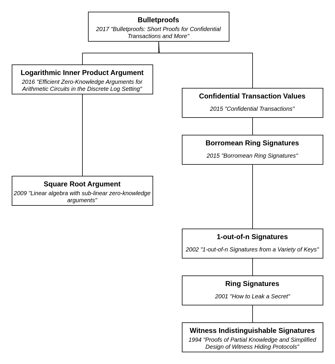
Note that this Tech-Tree omits detailed dependencies to maintain readability.

References

[1]

Bünz, B., Bootle, J., Boneh, D., Poelstra, A., Wuille, P. and Maxwell, G., 2018, May. Bulletproofs: Short proofs for confidential transactions and more. In 2018 IEEE symposium on security and privacy (SP) (pp. 315-334). IEEE.

[2]

Greg Maxwell, 2016. Confidential transactions. https://people.xiph.org/~greg/confidential_values.txt (opens in a new tab)

[3]

Maxwell, G. and Poelstra, A., 2015. Borromean ring signatures. Accessed: Jun, 8, p.2019.

[4]

Bootle, J., Cerulli, A., Chaidos, P., Groth, J. and Petit, C., 2016. Efficient zero-knowledge arguments for arithmetic circuits in the discrete log setting. In Advances in Cryptology–EUROCRYPT 2016: 35th Annual International Conference on the Theory and Applications of Cryptographic Techniques, Vienna, Austria, May 8-12, 2016, Proceedings, Part II 35 (pp. 327-357). Springer Berlin Heidelberg.

[5]

dalek cryptography, Cathie Yun, 2020. https://doc-internal.dalek.rs/bulletproofs/ (opens in a new tab)

[6]

Benedikt Bünz (Stanford University), May, 2018. Bulletproofs: Short Proofs for Confidential Transactions and More. IEEE Symposium on Security and Privacy YouTube channel. https://www.youtube.com/watch?v=Adrh6BCc_Ao (opens in a new tab)

[7]

Cathie Yun, June, 2018. Cathie Yun on Bulletproofs: Short Proofs for Confidential Transactions and More [PWL SF] 3/2018. PapersWeLove San Francisco Chapter YouTube channel. https://www.youtube.com/watch?v=BBe1JzUxSB8 (opens in a new tab)

[8]

Benedikt Bünz (https://crypto.stanford.edu/~buenz/ (opens in a new tab)), April, 2018. Benedikt Bünz : Bulletproofs. SF Bitcoin Developers YouTube Channel. https://www.youtube.com/watch?v=gMI8dkwGGcw (opens in a new tab)

[9]

Hoffmann, M., Klooß, M. and Rupp, A., 2019, November. Efficient zero-knowledge arguments in the discrete log setting, revisited. In Proceedings of the 2019 ACM SIGSAC Conference on Computer and Communications Security (pp. 2093-2110).

[10]

Mary Maller (Ethereum Foundation), May, 2021. Inner Product Arguments - Mary Maller. ZKProof Standards YouTube Channel. https://www.youtube.com/watch?v=dD_0Vn4BhmI (opens in a new tab)

[11]

Mary Maller (Ethereum Foundation), August, 2020. Mary Maller- "Inner Product Arguments". For IC3 Blockchain Camp 2020 on IC3 Initiative for Cryptocurrencies and Contracts YouTube channel. https://www.youtube.com/watch?v=Ne3XpSdMmzM (opens in a new tab)